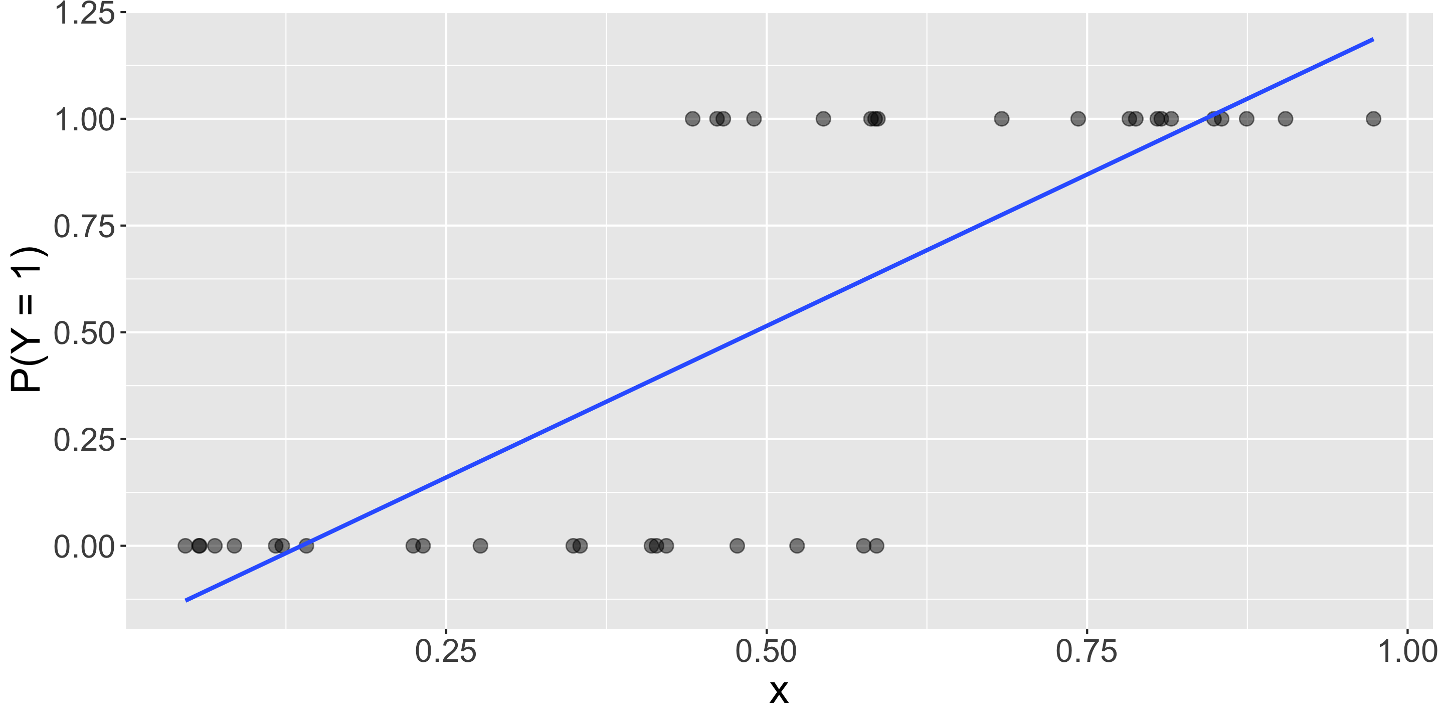
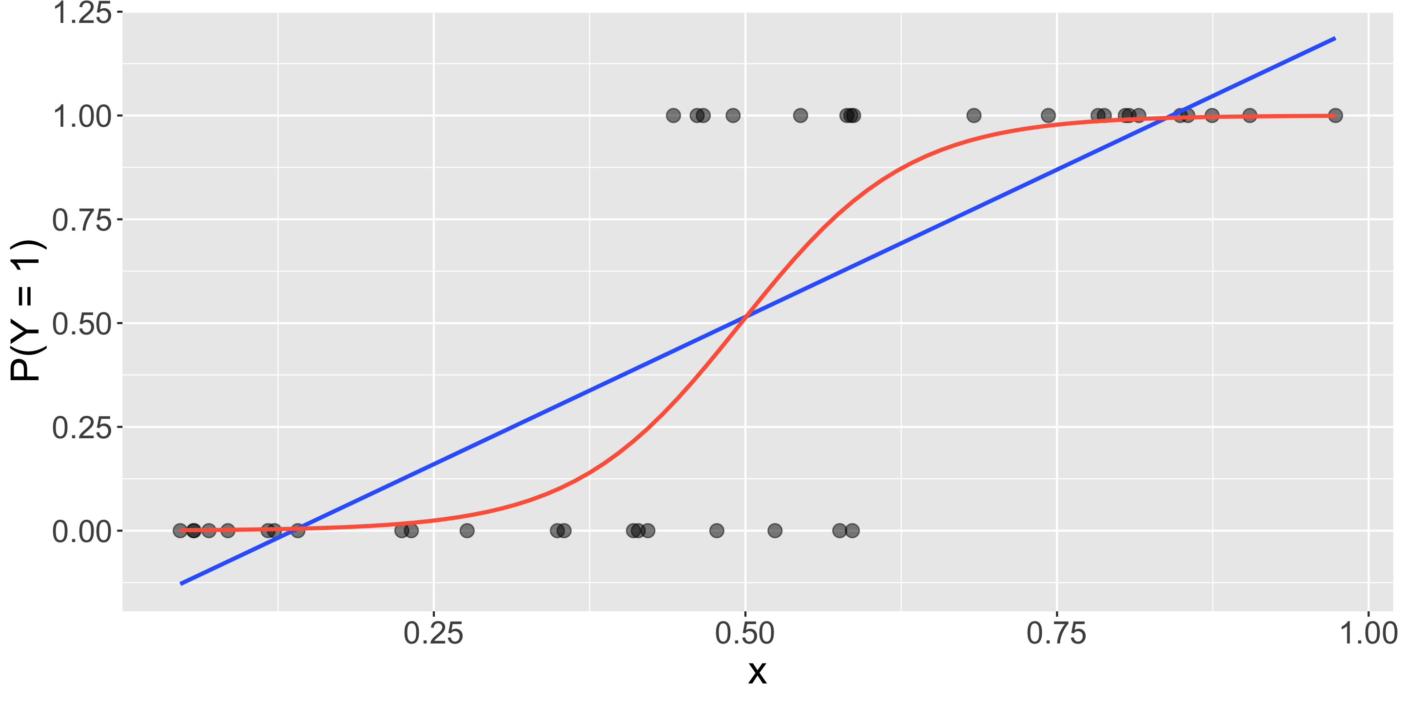
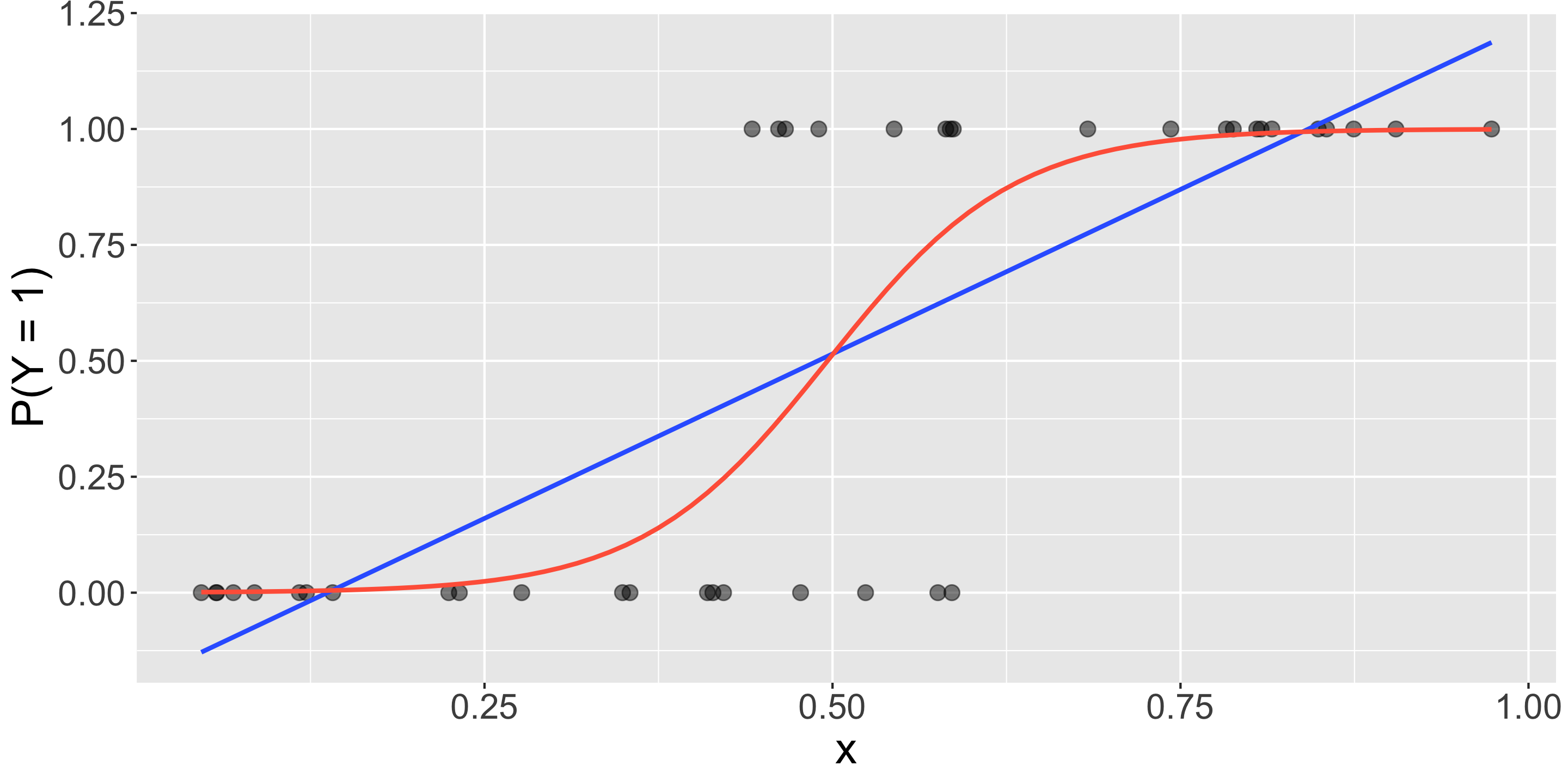
Question : How do we fit the model (the red curve) in R?
Logistic Regression Model in R
Instead of a linear regression model, let’s fit a logistic regression model to the Donner Party data!
library (broom)<- glm (Survived ~ Sex, data = donner, family = "binomial" )tidy (mod)
# A tibble: 2 × 5
  term        estimate std.error statistic p.value
  <chr>          <dbl>     <dbl>     <dbl>   <dbl>
1 (Intercept)    0.693     0.548      1.27  0.206
2 SexMale       -1.39      0.671     -2.07  0.0388
Fitted model: \[
\log\left(\frac{P(Y = 1)}{1 - P(Y = 1)} \right) = 0.693 - 1.386 x_{Sex:Male}
\]
But what do the coefficient estimates \(\hat{\beta}_0 = 0.693\) and \(\hat{\beta}_1 = - 1.386\) represent?
Interpretation of Coefficients
What do the coefficient estimates \(\hat{\beta}_0 = 0.693\) and \(\hat{\beta}_1 = - 1.386\) represent?
When Sex = “Female”:
\[\begin{align*}
\log\left(\frac{P(Y = 1)}{1 - P(Y = 1)} \right) &= \log (\text{odds}) \\
& = 0.693 \\
&= \hat\beta_0
\end{align*}\]
Therefore, \(\hat\beta_0\) represents the \(\log\) of the odds of survival for the baseline group.
When Sex = “Male”:
\[\begin{align*}
\log\left(\frac{P(Y = 1)}{1 - P(Y = 1)} \right) &= \log (\text{odds}) \\
&= 0.693 - 1.386 \\
&= \hat\beta_0 + \hat\beta_1
\end{align*}\]
Therefore, \(\hat\beta_1\) represents the change in the \(\log\) odds of survival when comparing the baseline group (Female) to Male.
Is there a more intuitive way to interpret logistic regression coefficients?
Interpretation of Coefficients
Recall the (2) following definitions:
(1) Odds:
\[\text{odds} = \frac{\text{prob of success}}{\text{prob of failure}} = \frac{P(Y = 1)}{1 - P(Y = 1)}\]
and (2) the logistic regression model :
\[\log\left(\frac{P(Y = 1)}{1 - P(Y = 1)}\right) = \beta_0 + \beta_1 x_1\]
So then
\[\text{odds} = \exp\left(\beta_0 + \beta_1 x_1\right)\]
Interpretation of Coefficients
(Estimated) odds of survival for female members of the Donner Party:
\[\exp\left(\hat{\beta}_0\right)\]
(Estimated) odds of survival for male members of the Donner Party:
\[\exp\left(\hat{\beta}_0 + \hat{\beta}_1\right)\]
What about interpreting \(\hat\beta_1\) on it’s own?
Interpretation of Coefficients
New concept:
Odds ratio : Comparison of odds between two groups
\[\text{odds ratio} = \frac{\text{odds of group 1}}{\text{odds of group 2}}\]
Interpretation of odds ratio: The odds of success in group 1 are ___ times the odds of success in group 2.
Note: Also useful property:
\[\exp(a + b) = \exp(a) \exp(b)\]
Interpretation of Coefficients
Computing the odds ratio:
\[\frac{\exp\left(\hat{\beta}_0 + \hat{\beta}_1 \right)}{\exp\left(\hat{\beta}_0 \right)} = \frac{\exp(\hat{\beta}_0)\exp(\hat{\beta}_1 )}{\exp(\hat{\beta}_0)} = \exp(\hat{\beta}_1)\]
Interpretation of Coefficients
How do we interpret \(\hat{\beta}_1 = - 1.386\) ?
\[\exp(\hat{\beta}_1) = \frac{\text{odds of survival if male} }{\text{odds of survival if female }}\]
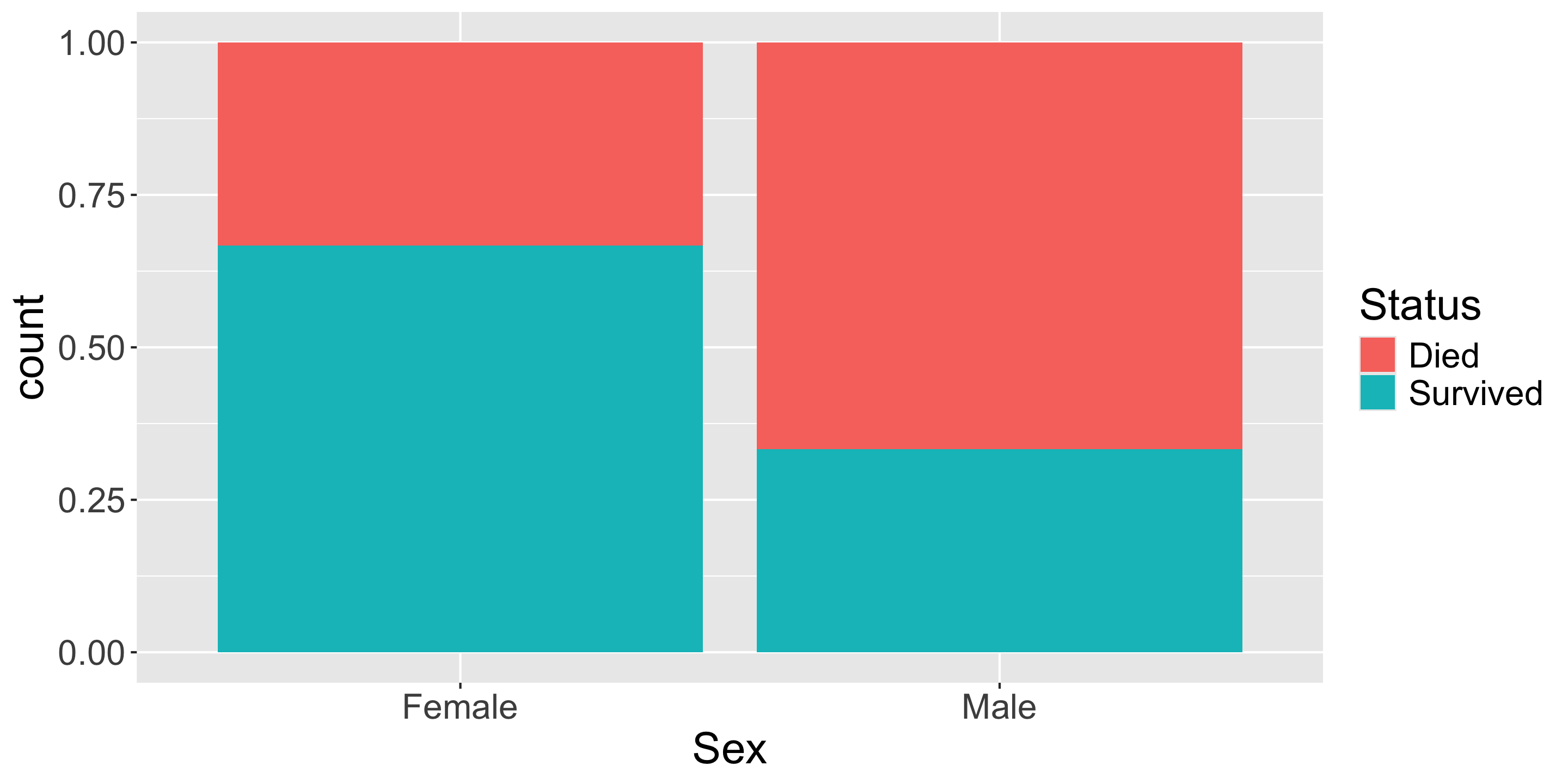
The estimated odds of survival for female members of the Donner Party are about 4 times that of male members!
What about quantitative predictors?
A new model
library (broom)<- glm (Survived ~ Sex + Age, data = donner, family = "binomial" )tidy (mod2)
# A tibble: 3 × 5
  term        estimate std.error statistic p.value
  <chr>          <dbl>     <dbl>     <dbl>   <dbl>
1 (Intercept)   3.23      1.39        2.33  0.0198
2 SexMale      -1.60      0.755      -2.11  0.0345
3 Age          -0.0782    0.0373     -2.10  0.0359
Interpretation of \(\hat\beta_1 = -1.597\) ?
The estimated odds of survival for female members of the Donner Party is nearly 5 times that of male members, holding age constant.
Interpretation of \(\hat\beta_2 = -0.078\) ?
Interpretation of Coefficients
(Estimated) odds of survival for \(x_{age} = t\) years:
\[\exp\left(\hat{\beta}_0 + \hat{\beta}_1 x_{1} + \hat{\beta}_2 t\right)\]
(Estimated) odds of survival for \(x_{age} = t + 1\) years:
\[\exp\left(\hat{\beta}_0 + \hat{\beta}_1 x_1 + \hat{\beta}_2 (t + 1)\right)\]
odds ratio:
\[\frac{\exp\left(\hat{\beta}_0 + \hat{\beta}_1 x_{1} + \hat{\beta}_2 (t + 1)\right)}{\exp\left(\hat{\beta}_0 + \hat{\beta}_1 x_{1} + \hat{\beta}_2 t\right)} = \frac{\exp\left(\hat{\beta}_0\right)\exp\left(\hat{\beta}_1 x_{1}\right) \exp\left(\hat\beta_2 (t + 1)\right)}{\exp\left(\hat{\beta}_0\right)\exp\left(\hat{\beta}_1 x_{1}\right) \exp\left(\hat\beta_2 t\right)} = \exp(\hat{\beta}_2)\]
Interpretation of Coefficients
How do we interpret \(\hat{\beta}_2 = -0.078\) ?
\[\exp(\hat{\beta}_2) = \frac{\text{odds of surviving at age } (t + 1)}{\text{odds of surviving at age t}}\]
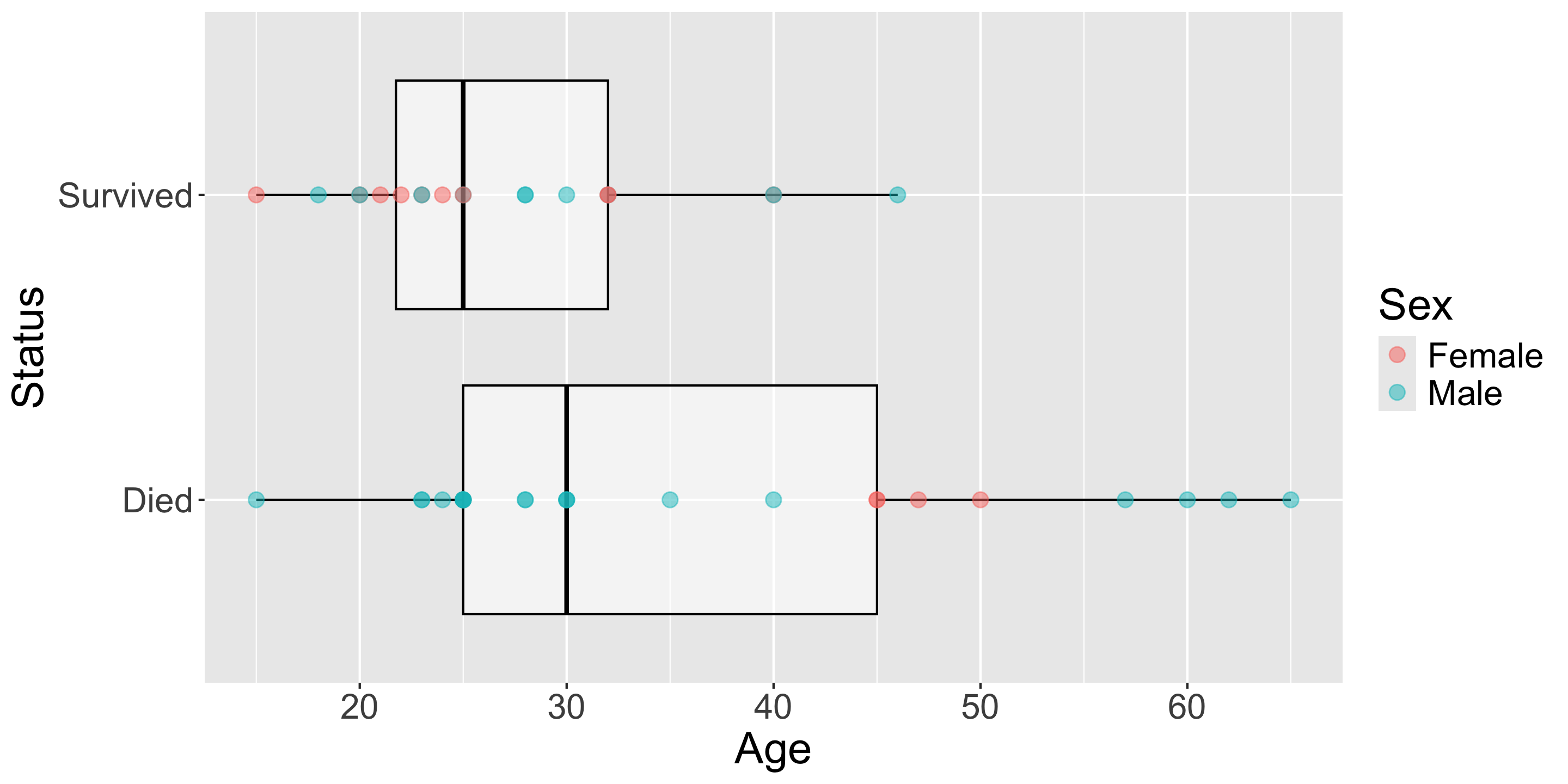
Holding sex constant, for a 1 year increase in age, the estimated odds of survival are multiplied by 0.925.
Prediction
How can I use this model to predict, for a given sex and age:
the odds of survival,
the probability of survival, and
whether or not we expect survival?
Prediction
How can I use this model to predict, for a given sex and age:
the odds of survival ,the probability of survival, and
whether or not we expect survival?
\[
\text{odds} = \frac{P(Y = 1)}{1 - P(Y = 1)} = \exp\left(\hat\beta_0 + \hat\beta_1x_1 + \hat\beta_2x_2\right)
\]
In R:
<- exp (predict (mod2, newdata = data.frame (Age = c (20 , 65 ),Sex = c ("Female" , "Male" )))
         1          2
5.29272036 0.03174105
Prediction
How can I use this model to predict, for a given sex and age:
the odds of survival,
the probability of survival , andwhether or not we expect survival?
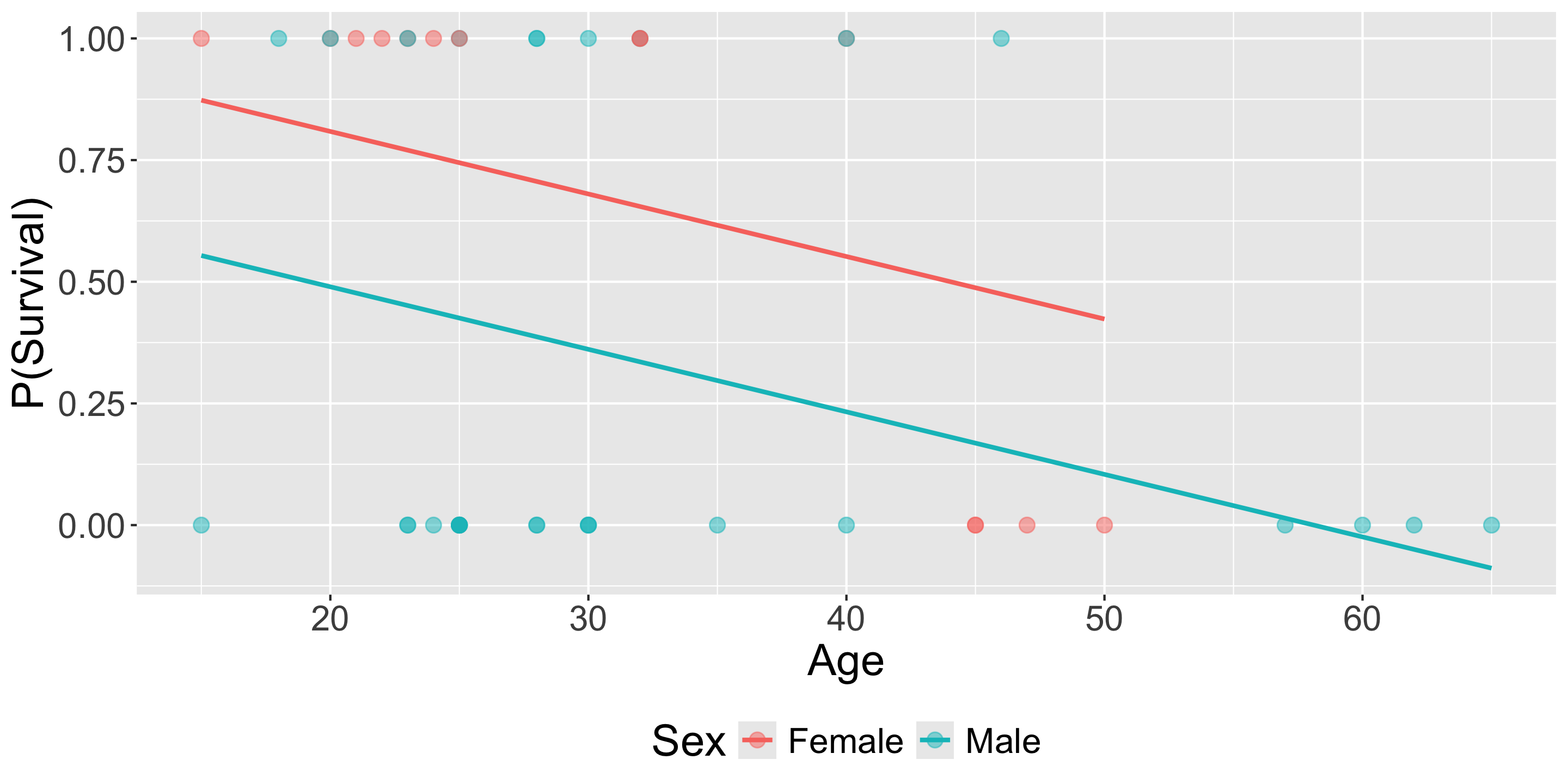
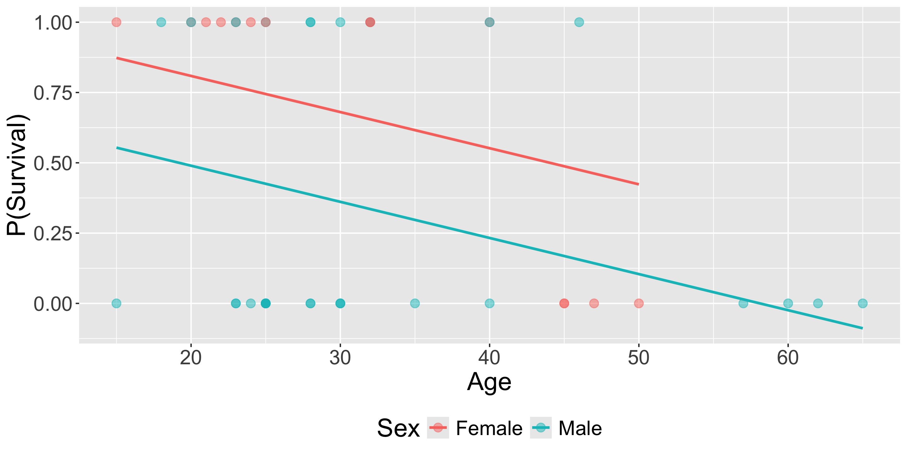
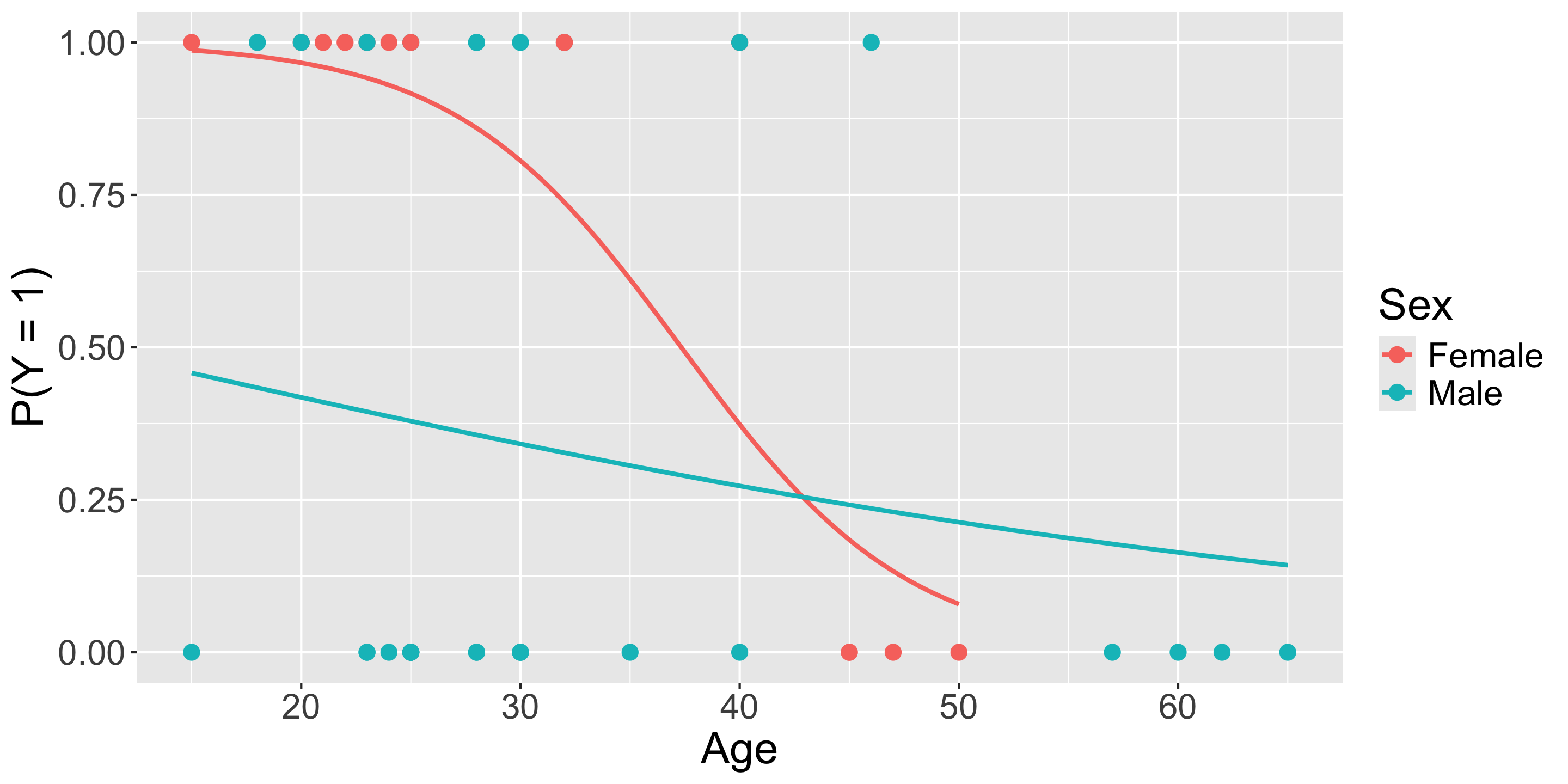
ggplot (donner, aes (x = Age,y = Survived, color = Sex)) + geom_point (size = 3 ) + labs (y = "P(Y = 1)" ) + geom_smooth (method = 'glm' ,method.args = list (family = "binomial" ),se = FALSE )
Prediction
How can I use this model to predict, for a given sex and age:
the odds of survival,
the probability of survival , andwhether or not we expect survival?
\[
P(Y = 1) = \frac{\exp\left(\hat\beta_0 + \hat\beta_1x_1 + \hat\beta_2x_2\right)}{1 + \exp\left(\hat\beta_0 + \hat\beta_1x_1 + \hat\beta_2x_2\right)}
\]
In R:
<- odds / (1 + odds)
         1          2
0.84108622 0.03076455
# or <- predict (mod2,newdata = data.frame (Age = c (20 , 65 ),Sex = c ("Female" , "Male" )), type = "response" )
         1          2
0.84108622 0.03076455
Prediction
How can I use this model to predict, for a given sex and age:
the odds of survival,
the probability of survival, and
whether or not we expect survival ?
We can use the predicted probability at for an individual to help us predict the binary outcome .
\[\widehat{P(Y = 1)} \geq 0.5 \rightarrow \hat{y} = 1\] \[\widehat{P(Y = 1)} < 0.5 \rightarrow \hat{y} = 0\]
Predicted probability of survival for each member of the Donner Party
<- predict (mod2, newdata = donner, type = "response" )head (preds)
        1         2         3         4         5         6
0.4587010 0.5255405 0.1831661 0.3289359 0.3643360 0.1831661
Prediction Accuracy
%>% bind_cols (preds = preds) %>% # quickly add as a column mutate (pred_survived = case_when (>= 0.5 ~ 1 ,< 0.5 ~ 0 %>% group_by (Survived) %>% count (pred_survived)
# A tibble: 4 × 3
# Groups:   Survived [2]
  Survived pred_survived     n
     <dbl>         <dbl> <int>
1        0             0    23
2        0             1     2
3        1             0     8
4        1             1    12
Pretty good!
How should we quantify our error rates?
Recap
Today, we learned about logistic regression , a model suitable when your response variable is categorical and binary , but your predictors can be categorical or quantitative .
Logistic regression is similar to linear regression, but we link the response variable to the linear predictor with the log odds or “logit” function:
\[
\log\left(\frac{P(Y = 1)}{1 - P(Y = 1)} \right) = \beta_0 + \beta_1 x_1 + \beta_2 x_2 + \cdots + \beta_p x_p
\]
Unlike linear regression models, logistic regression models always predict the probability of success to be between 0 and 1 .
We have to interpret odds and odds ratios to interpret the coefficients.
We can predict many quantities: odds of success, probability of success, and even whether or not we expect success!