spc_tbl_ [47 × 31] (S3: spec_tbl_df/tbl_df/tbl/data.frame)
 $ Functional   : chr [1:47] "Typ" "Typ" "Typ" "Typ" ...
 $ BldgType     : chr [1:47] "1Fam" "1Fam" "1Fam" "TwnhsE" ...
 $ Foundation   : chr [1:47] "CBlock" "PConc" "CBlock" "CBlock" ...
 $ LotShape     : chr [1:47] "Reg" "Reg" "IR1" "IR1" ...
 $ LandSlope    : chr [1:47] "Gtl" "Gtl" "Gtl" "Gtl" ...
 $ SaleCondition: chr [1:47] "Normal" "Normal" "Normal" "Normal" ...
 $ RoofMatl     : chr [1:47] "CompShg" "CompShg" "CompShg" "CompShg" ...
 $ ScreenPorch  : num [1:47] 0 0 0 0 0 0 0 0 0 0 ...
 $ MSSubClass   : num [1:47] 20 20 20 120 30 20 50 30 60 20 ...
 $ GarageCars   : num [1:47] 2 0 0 2 1 1 1 1 2 2 ...
 $ Id           : num [1:47] 2 90 100 127 155 207 240 269 281 339 ...
 $ BedroomAbvGr : num [1:47] 3 3 3 2 4 3 3 2 3 3 ...
 $ TotalBsmtSF  : num [1:47] 1262 990 950 1078 1200 ...
 $ LotArea      : num [1:47] 9600 8070 9320 4928 11340 ...
 $ OpenPorchSF  : num [1:47] 0 0 0 205 0 30 140 25 84 45 ...
 $ BsmtFullBath : num [1:47] 0 1 1 0 0 0 0 0 0 1 ...
 $ WoodDeckSF   : num [1:47] 298 0 352 0 0 0 0 0 0 108 ...
 $ OverallCond  : num [1:47] 8 5 5 5 5 5 4 6 6 7 ...
 $ YrSold       : num [1:47] 2007 2007 2010 2007 2006 ...
 $ GrLivArea    : num [1:47] 1262 990 1225 958 1200 ...
 $ MoSold       : num [1:47] 5 8 1 2 3 3 4 2 1 5 ...
 $ TotRmsAbvGrd : num [1:47] 6 5 6 5 7 8 7 4 7 8 ...
 $ PoolArea     : num [1:47] 0 0 0 0 0 0 0 0 0 0 ...
 $ YearBuilt    : num [1:47] 1976 1994 1959 1976 1923 ...
 $ GarageArea   : num [1:47] 460 0 0 440 312 349 220 924 575 440 ...
 $ OverallQual  : num [1:47] 6 4 4 6 6 5 6 5 7 7 ...
 $ Fireplaces   : num [1:47] 1 0 0 1 0 1 1 1 1 0 ...
 $ SalePrice    : num [1:47] 181500 123600 128950 128000 125000 ...
 $ EnclosedPorch: num [1:47] 0 0 0 0 228 0 0 0 0 0 ...
 $ FullBath     : num [1:47] 2 1 1 2 1 1 1 1 2 2 ...
 $ HalfBath     : num [1:47] 0 0 1 0 0 1 1 0 1 0 ...
 - attr(*, "spec")=
  .. cols(
  ..   Functional = col_character(),
  ..   BldgType = col_character(),
  ..   Foundation = col_character(),
  ..   LotShape = col_character(),
  ..   LandSlope = col_character(),
  ..   SaleCondition = col_character(),
  ..   RoofMatl = col_character(),
  ..   ScreenPorch = col_double(),
  ..   MSSubClass = col_double(),
  ..   GarageCars = col_double(),
  ..   Id = col_double(),
  ..   BedroomAbvGr = col_double(),
  ..   TotalBsmtSF = col_double(),
  ..   LotArea = col_double(),
  ..   OpenPorchSF = col_double(),
  ..   BsmtFullBath = col_double(),
  ..   WoodDeckSF = col_double(),
  ..   OverallCond = col_double(),
  ..   YrSold = col_double(),
  ..   GrLivArea = col_double(),
  ..   MoSold = col_double(),
  ..   TotRmsAbvGrd = col_double(),
  ..   PoolArea = col_double(),
  ..   YearBuilt = col_double(),
  ..   GarageArea = col_double(),
  ..   OverallQual = col_double(),
  ..   Fireplaces = col_double(),
  ..   SalePrice = col_double(),
  ..   EnclosedPorch = col_double(),
  ..   FullBath = col_double(),
  ..   HalfBath = col_double()
  .. )
- attr(*, "problems")=<externalptr> 
Regression Competition
Grayson White
Stat 243
Week 7 | Fall 2026
Announcements
- Don’t forget about Group Project Assignment 1!
- Deadline to turn in the proposal for priority feedback is this Friday, 10/16.
Goals for this week
Monday:
- Ultimate regression competition showdown!!!
Wednesday:
- \(k\)NN
Friday:
- Quiz on penalized regression.
- I have decided to not assign a Lab on Friday!
Regression Competition
Regression Competition
- We will have a 12-player single-elimination bracket style competition, based on your “best” model from Lab 4.
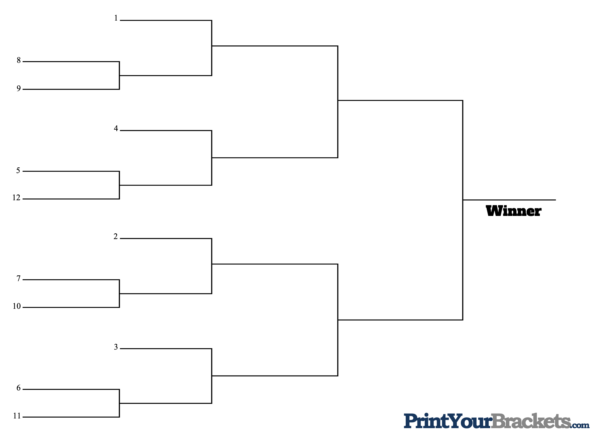
Seeding: Stat Learning Trivia

Round 1
Seeding: Stat Learning Trivia (1)
Unsupervised learning refers to a type of statistical learning without
- any continuous variables
- a quantitative response variable
- any auxiliary variables
- any response variables
Seeding: Stat Learning Trivia (2)
Bootstrapping is useful for …
- Improving predictive performance
- Estimating a statistic’s center
- Estimating a statistic’s variation
- None of the above
Seeding: Stat Learning Trivia (3)
TRUE or FALSE: Penalized regression can decrease overall MSE by decreasing bias and increasing variance
Seeding: Stat Learning Trivia (4)
As \(n\to\infty\), the probability that the \(j\)th observation is not in the bootstrap sample is:
- \(e^{-1}\)
- \(-e\)
- \(\frac{1}{e}\)
- Both (a) and (c)
Seeding: Stat Learning Trivia (5)
The average test MSE can be decomposed into what three terms?
- bias(\(\hat f\)), variance(\(\hat f\)), variance(\(\epsilon\))
- bias\(^2\)(\(\hat f\)), variance\(^2\)(\(\hat f\)), variance(\(\epsilon\))
- bias\(^2\)(\(\hat f\)), variance(\(\hat f\)), variance(\(\epsilon\))
- Mean, Squared, and Error
Seeding: Stat Learning Trivia (6)
MAD, MSE, and MZOL are all examples of what?
- regression functions
- step functions
- loss functions
- found functions
Round 2
If you “won” in Round 1 you are in Round 2.
Seeding: Stat Learning Trivia (7)
What penalization method also performs variable selection?
Seeding: Stat Learning Trivia (8)
A model with low training RSS, but high testing RSS might be doing what to the training data?
Seeding: Stat Learning Trivia (9)
Suppose you have 160 training observations and choose to perform 10-fold cross validation. How many observations will be in each fold?
Final Round
If you “lost” in Round 2 you are in the Final Round.
Seeding: Stat Learning Trivia (10)
How many authors are there for our main textbook, ISLR (Second Edition)?
Competition time!
Training and testing data
spc_tbl_ [150 × 31] (S3: spec_tbl_df/tbl_df/tbl/data.frame)
 $ Functional   : chr [1:150] "Typ" "Min1" "Typ" "Typ" ...
 $ BldgType     : chr [1:150] "1Fam" "1Fam" "1Fam" "1Fam" ...
 $ Foundation   : chr [1:150] "PConc" "Slab" "PConc" "BrkTil" ...
 $ LotShape     : chr [1:150] "IR1" "Reg" "IR1" "Reg" ...
 $ LandSlope    : chr [1:150] "Gtl" "Gtl" "Gtl" "Gtl" ...
 $ SaleCondition: chr [1:150] "Normal" "Normal" "Normal" "Normal" ...
 $ RoofMatl     : chr [1:150] "CompShg" "CompShg" "CompShg" "CompShg" ...
 $ ScreenPorch  : num [1:150] 0 0 0 0 0 0 0 0 0 0 ...
 $ MSSubClass   : num [1:150] 60 20 60 50 20 20 60 20 20 20 ...
 $ GarageCars   : num [1:150] 3 2 2 2 2 1 2 2 1 2 ...
 $ Id           : num [1:150] 1418 1049 821 946 423 ...
 $ BedroomAbvGr : num [1:150] 3 3 3 2 2 3 3 3 3 2 ...
 $ TotalBsmtSF  : num [1:150] 1284 0 798 1088 988 ...
 $ LotArea      : num [1:150] 16545 21750 7226 8820 21750 ...
 $ OpenPorchSF  : num [1:150] 126 0 45 0 0 0 111 32 319 33 ...
 $ BsmtFullBath : num [1:150] 1 0 0 0 0 1 1 0 1 0 ...
 $ WoodDeckSF   : num [1:150] 0 0 0 48 0 289 306 222 0 120 ...
 $ OverallCond  : num [1:150] 5 4 5 6 5 6 5 7 6 5 ...
 $ YrSold       : num [1:150] 2009 2009 2008 2009 2008 ...
 $ GrLivArea    : num [1:150] 2450 1771 1640 1869 988 ...
 $ MoSold       : num [1:150] 5 11 6 9 2 4 7 5 1 12 ...
 $ TotRmsAbvGrd : num [1:150] 7 9 6 7 4 6 6 5 6 6 ...
 $ PoolArea     : num [1:150] 0 0 0 0 0 0 0 0 0 0 ...
 $ YearBuilt    : num [1:150] 1998 1960 2003 1890 1954 ...
 $ GarageArea   : num [1:150] 1069 336 595 456 520 ...
 $ OverallQual  : num [1:150] 8 5 7 5 5 6 6 5 5 8 ...
 $ Fireplaces   : num [1:150] 1 1 0 0 0 1 1 0 0 1 ...
 $ SalePrice    : num [1:150] 340000 115000 183000 124900 113000 ...
 $ EnclosedPorch: num [1:150] 0 0 0 244 0 0 0 0 0 0 ...
 $ FullBath     : num [1:150] 2 1 2 1 1 2 2 1 1 2 ...
 $ HalfBath     : num [1:150] 1 0 1 0 0 0 1 0 0 0 ...
 - attr(*, "spec")=
  .. cols(
  ..   Functional = col_character(),
  ..   BldgType = col_character(),
  ..   Foundation = col_character(),
  ..   LotShape = col_character(),
  ..   LandSlope = col_character(),
  ..   SaleCondition = col_character(),
  ..   RoofMatl = col_character(),
  ..   ScreenPorch = col_double(),
  ..   MSSubClass = col_double(),
  ..   GarageCars = col_double(),
  ..   Id = col_double(),
  ..   BedroomAbvGr = col_double(),
  ..   TotalBsmtSF = col_double(),
  ..   LotArea = col_double(),
  ..   OpenPorchSF = col_double(),
  ..   BsmtFullBath = col_double(),
  ..   WoodDeckSF = col_double(),
  ..   OverallCond = col_double(),
  ..   YrSold = col_double(),
  ..   GrLivArea = col_double(),
  ..   MoSold = col_double(),
  ..   TotRmsAbvGrd = col_double(),
  ..   PoolArea = col_double(),
  ..   YearBuilt = col_double(),
  ..   GarageArea = col_double(),
  ..   OverallQual = col_double(),
  ..   Fireplaces = col_double(),
  ..   SalePrice = col_double(),
  ..   EnclosedPorch = col_double(),
  ..   FullBath = col_double(),
  ..   HalfBath = col_double()
  .. )
 - attr(*, "problems")=<externalptr>
Your models
List of 2
 $ models:List of 12
  ..$ Ellarain_Moore_model    :function (training_data, testing_data)
  ..$ Brendan_Fingal_model    :function (training_data, testing_data)
  ..$ Tate_Beech_model        :function (training_data, testing_data)
  ..$ Dane_Vaughn_model       :function (training_data, testing_data)
  ..$ Cassia_Post_model       :function (training_data, testing_data)
  ..$ Schwa_Yeleti_model      :function (training_data, testing_data)
  ..$ Jaden_Bauer_model       :function (training_data, testing_data)
  ..$ Anne_Heissenbuttel_model:function (training_data, testing_data)
  ..$ Ida_Landecker_model     :function (training_data, testing_data)
  ..$ Kaishin_Lin_model       :function (training_data, testing_data)
  ..$ Fuxing_Lu_model         :function (training_data, testing_data)
  ..$ Eleanor_Tonn_model      :function (training_data, testing_data)
$ seeds : num [1:12] 6 8 12 10 11 9 7 2 5 4 ...function (training_data, testing_data)
{
my_mod <- lm(SalePrice ~ OverallQual + GrLivArea + TotalBsmtSF +
YearBuilt, data = training_data)
predict(my_mod, testing_data)
}[1] 6Compete!
compete <- function(seeds, training_data, testing_data, print_rmse) {
  indx1 <- which(competition$seeds == seeds[1])
  indx2 <- which(competition$seeds == seeds[2])

  indx1_preds <- competition$models[[indx1]](training_data, testing_data)
  indx2_preds <- competition$models[[indx2]](training_data, testing_data)

  rmse1 <- sqrt(mean( (indx1_preds - testing_data$SalePrice)^2 ))
  rmse2 <- sqrt(mean( (indx2_preds - testing_data$SalePrice)^2 ))

  if (print_rmse) {
    if (rmse1 < rmse2) {
      print(paste0("Seed ", seeds[1], " wins with an RMSE of ", round(rmse1, 2),
                   " compared to Seed ", seeds[2], "'s RMSE of ", round(rmse2, 2)))
    } else if (rmse1 > rmse2) {
      print(paste0("Seed ", seeds[2], " wins with an RMSE of ", round(rmse2, 2),
               " compared to Seed ", seeds[1], "'s RMSE of ", round(rmse1, 2)))
    } else {
      print("Tie!")
    }
  }

  if (!print_rmse) {
    if (rmse1 < rmse2) {
      print(paste0("Seed ", seeds[1], " wins!"))
    } else if (rmse1 > rmse2) {
      print(paste0("Seed ", seeds[2], " wins!"))
    } else {
      print("Tie!")
    }
  }


}
The Play-in
The Play-in
In order to induce some randomness into the tournament, at each phase, we will first take a bootstrap sample of our testing data.
In the “finals” we will use the original (non-bootstrapped) sample.
Play-in: Game 1
Play-in: Game 1
Play-in: Game 2
Play-in: Game 2
Play-in: Game 3
Play-in: Game 3
Play-in: Game 4
Play-in: Game 4
Round 1
Round 1: Game 1
Round 1: Game 1
Round 1: Game 2
Round 1: Game 2
Round 1: Game 3
Round 1: Game 3
Round 1: Game 4
Round 1: Game 4
Round 2
Round 2: Game 1
Round 2: Game 1
Round 2: Game 2
Round 2: Game 2
The Finals
The Finals
The Finals
Most unbiased predictions
compete_bias <- function(seeds, training_data, testing_data) {
  indx1 <- which(competition$seeds == seeds[1])
  indx2 <- which(competition$seeds == seeds[2])

  indx1_preds <- competition$models[[indx1]](training_data, testing_data)
  indx2_preds <- competition$models[[indx2]](training_data, testing_data)

  bias1 <- mean( (indx1_preds - testing_data$SalePrice) )
  bias2 <- mean( (indx2_preds - testing_data$SalePrice) )

    if (abs(bias1) < abs(bias2)) {
      print(paste0("Seed ", seeds[1], " wins with an bias of ", round(bias1, 2),
                   " compared to Seed ", seeds[2], "'s bias of ", round(bias2, 2)))
    } else if (abs(bias1) > abs(bias2)) {
      print(paste0("Seed ", seeds[2], " wins with an bias of ", round(bias2, 2),
               " compared to Seed ", seeds[1], "'s bias of ", round(bias1, 2)))
    } else {
      print("Tie!")
    }


}
Most unbiased predictions
Next time
Lenny will discuss \(k\)NN.
On Friday, Marcus will administer and proctor the quiz.
See you after fall break!