03:00

Penalized Regression: LASSO
Grayson White
Stat 243
Week 6 | Fall 2026
Group Project Preferences. Please fill out the Google form by Thursday at 3pm.
More discussion of the group project scope on Friday.
Monday:
Introduce penalization to improve MSE in regression models
Define and apply Ridge Regression in a case study
Today:
Introduce LASSO as a penalization and variable selection method
Apply LASSO in a case study
Suppose we’ve selected a regression model: \[Y = \beta_0 + \beta_1X_1 + \dots + \beta_pX_p + \epsilon,\qquad \epsilon \sim N(0,~\sigma^2)\]
Least Squares: Find \(\beta\)s that minimize \[RSS=\sum_{i=1}^n\Big(Y_i - \hat{Y}_i\ \Big)^2\]
Ridge Regression: Find \(\beta\)s that minimize \[ \textrm{RSS} + \underbrace{\lambda\sum_{j = 1}^p \beta_j^2}_\text{Ridge Penalty} \qquad \textrm{where } \lambda \geq 0 \]
\[\begin{aligned} \text{Least Squares: }& \text{Minimize RSS}\\ \text{Ridge Regression: }& \text{Minimize RSS} + \lambda \sum_{j=1}^p \beta_j^2 \end{aligned}\]
Least Absolute Shrinkage and Selection Operator: Find \(\beta\)s that minimize \[ \textrm{RSS} + \underbrace{\lambda\sum_{j = 1}^p \big|\beta_j\big|}_\text{LASSO Penalty} \qquad \textrm{where } \lambda \geq 0 \]
Goal of LASSO Penalty: Make coefficients smaller
Like Ridge, LASSO increases bias but decreases variance and (hopefully) MSE.
So how is LASSO different from Ridge?
\[\begin{aligned} \text{Least Squares: }& \text{Minimize RSS}\\ \text{Ridge Regression: }& \text{Minimize RSS} + \lambda \sum_{j=1}^p \beta_j^2\\ \text{LASSO Regression: }& \text{Minimize RSS} + \lambda \sum_{j=1}^p \big|\beta_j\big| \end{aligned}\]
Suppose \(\beta_j= -10\). Calculate \(\beta_j^2\) and \(\big|\beta_j\big|\), then explain why this shows that Ridge penalizes “big” coefficients more than LASSO.
Suppose \(\beta_j= 0.1\). Calculate \(\beta_j^2\) and \(\big|\beta_j\big|\), then explain why this shows that LASSO penalizes “small” coefficients more than Ridge.
How much does each penalty decrease if \(\beta_j\) moves from \(10\) to \(9.9\)? What about from \(0.1\) to \(0\)?
Hypothesize why LASSO might shrink coefficients to exactly zero more often than Ridge.
03:00
We’ve just uncovered why LASSO is a variable “selection operator”:
Ridge and LASSO: Coefficients are encouraged to shrink.
Ridge: Penalty gets relatively smaller as coefficients get smaller
LASSO: Penalty gets relatively larger as coefficients get smaller
Bigger benefit of making small coefficients precisely 0.
\(\beta_j=0\) \(\implies\) \(X_j\) removed from model!
This is variable selection!
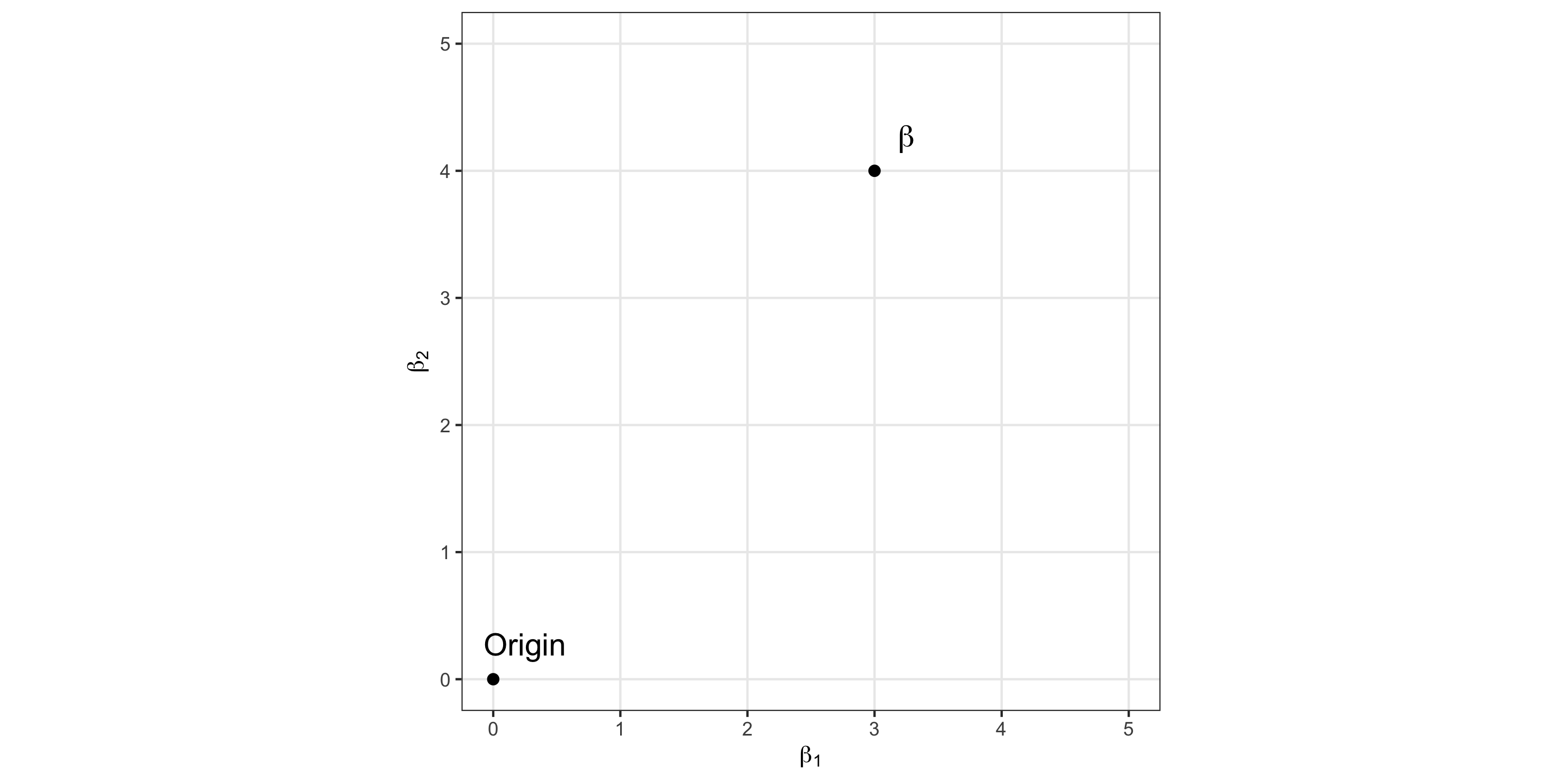
How to measure distance between a point \(x=(x_1, \dots, x_p)\) and the origin \((0, \dots, 0)\)?
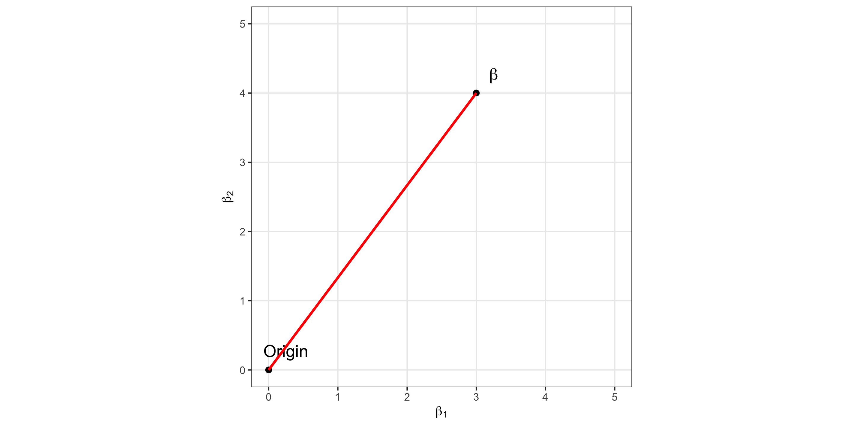
Euclidean distance: “straight line” distance: \[ \Vert x\Vert_2 = \sqrt{x_1^2 + \dots + x_p^2} = \sqrt{ \sum_{j=1}^p x_j^2} \]
Most common: Result of the Pythagorean theorem
Also called the \(\ell_2\) norm
Ridge uses \(\big(\Vert x\Vert_2\big)^2\) to “shrink” coefficients
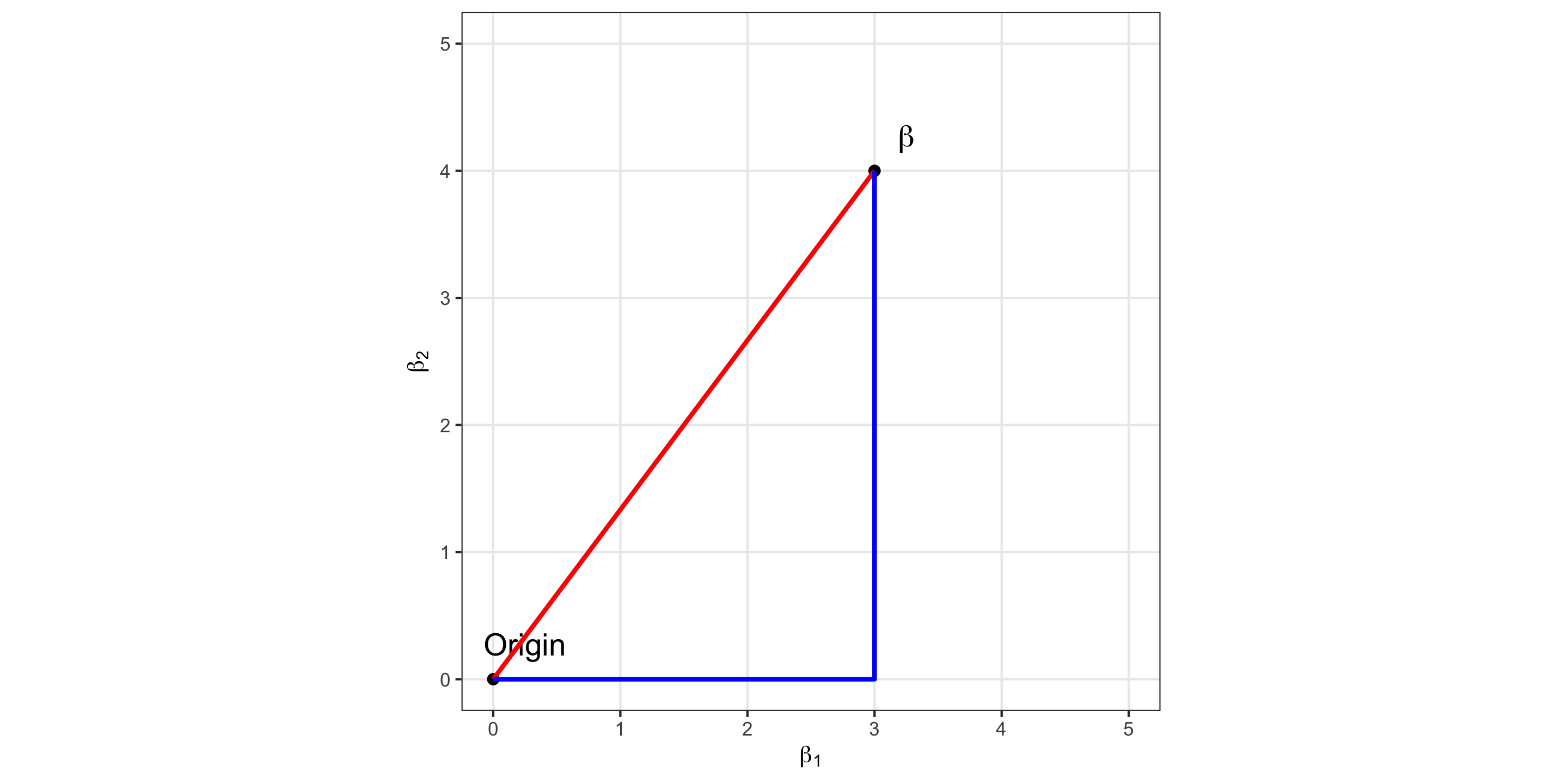
Manhattan distance: “grid line” distance: \[ \Vert x\Vert_1 = |x_1| + \dots + |x_p| = \sum_{j=1}^p |x_j| \]
the \(\ell_1\) norm
LASSO uses \(\Vert x\Vert_1\) directly for shrinkage


\(\Vert \beta \Vert_2 = \sqrt{3^2 + 4^2} = 5\)
\(\Vert \beta \Vert_1 = 3 + 4 = 7\)
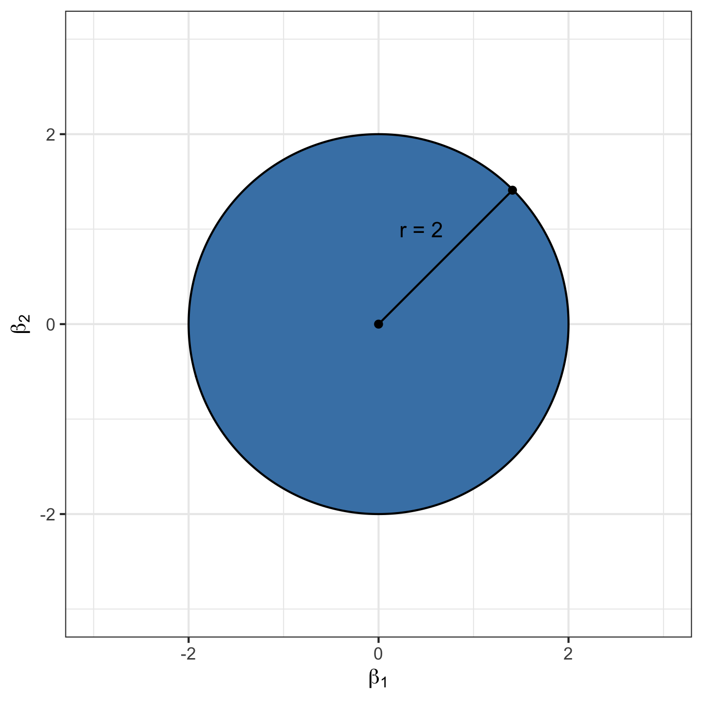
What does a circle of radius \(r\) look like in the \(\ell_2\) norm?
\[ \Vert \beta \Vert_2 = \sqrt{ \beta_1^2 + \beta_2^2 } \leq r \]
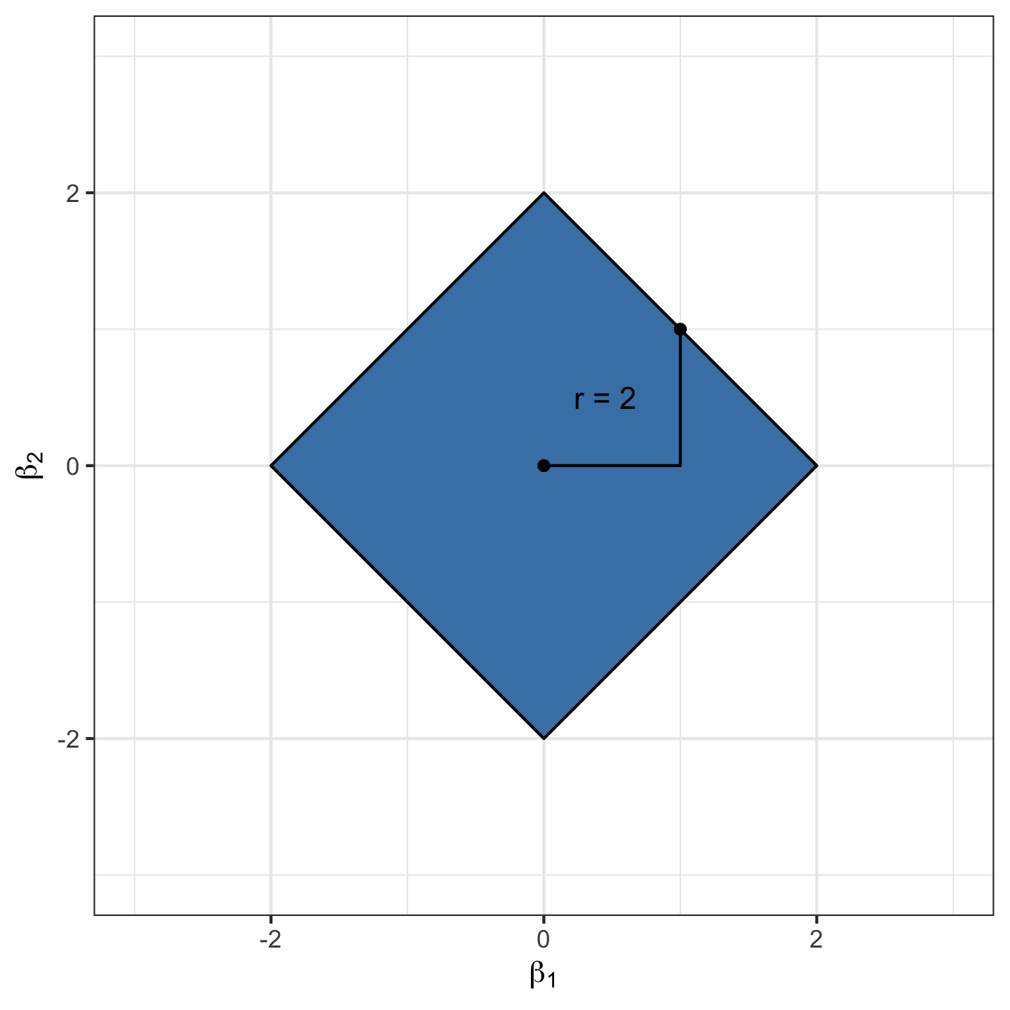
What does a “circle” of radius \(r\) look like in the \(\ell_1\) norm?
\[ \Vert \beta \Vert_1 = |\beta_1| + |\beta_2| \leq r \]
In ridge regression, we seek parameters \(\beta\) that minimize RSS plus the (squared) \(\ell_2\) norm of \(\beta\): \[ \textrm{RSS} + \lambda \sum_{i =1}^p \beta_i^2 = \mathrm{RSS} + \lambda\Vert\beta\Vert_2^2 \]
Alternatively, we could seek parameters \(\beta\) that minimize RSS plus the \(\ell_1\) norm of \(\beta\):
\[ \textrm{RSS} + \lambda \sum_{i =1}^p |\beta_i| = \mathrm{RSS} + \lambda \Vert \beta \Vert_1 \]
We have now reconstructed ridge and LASSO regression in terms of \(\ell_1\) and \(\ell_2\) norms!
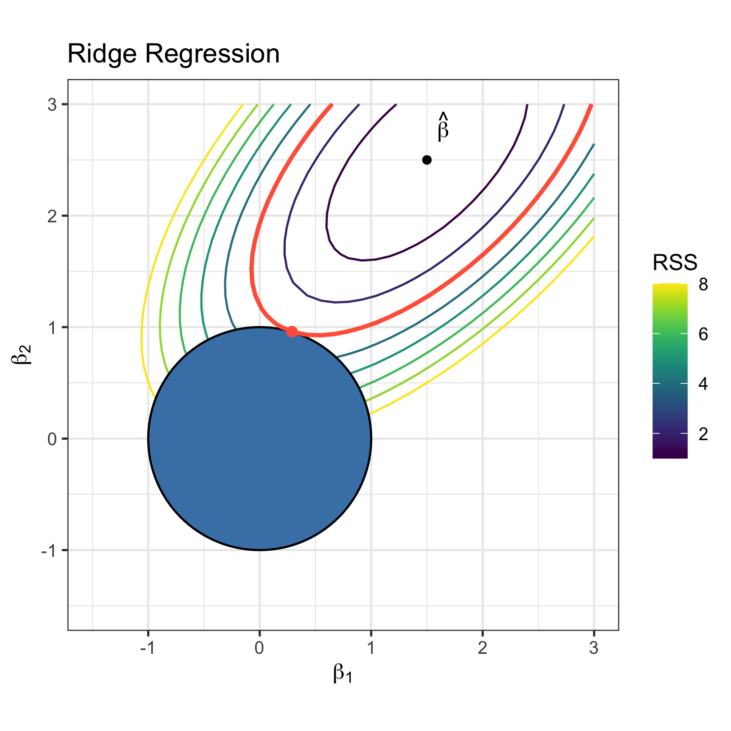
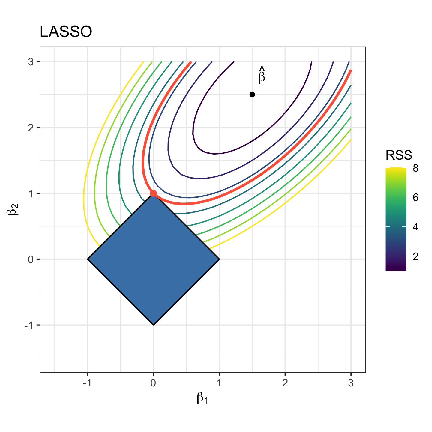
Instead of thinking of Ridge Regression and LASSO as minimizing the sum of RSS and the shrinkage penalty, we can think of them as solving a restricted optimization problem:
For each \(s \geq 0\), Ridge Regression seeks to minimize \(\textrm{RSS}\) subject to \(\Vert\beta\Vert_2^2 \leq s\)
For each \(s \geq 0\), LASSO seeks to minimize \(\textrm{RSS}\) subject to \(\Vert\beta\Vert_1 \leq s\)
Suppose \(q\) is \(1\) or \(2\). For each \(\lambda > 0\), there is exactly one \(s \geq 0\) so that if \(\beta\) minimizes \[ \textrm{RSS} + \lambda \Vert \beta \Vert_q^q \qquad \]
then \(\beta\) minimizes \[ \mathrm{RSS} \qquad \textrm{ subject to } \Vert \beta \Vert_q^q \leq s \]
For LASSO, the solution to the optimization problem often lies on a vertex of the domain, which corresponds to a subspace where one or more parameters are \(0\).
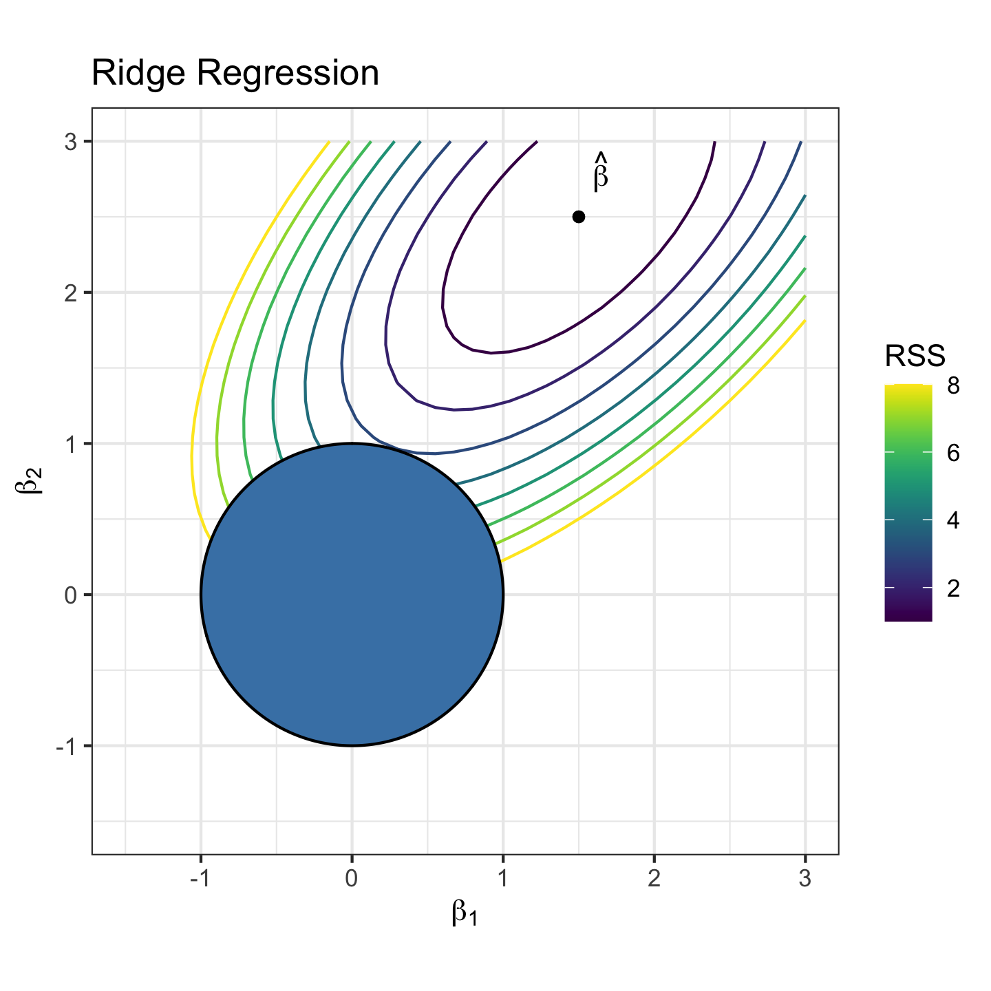
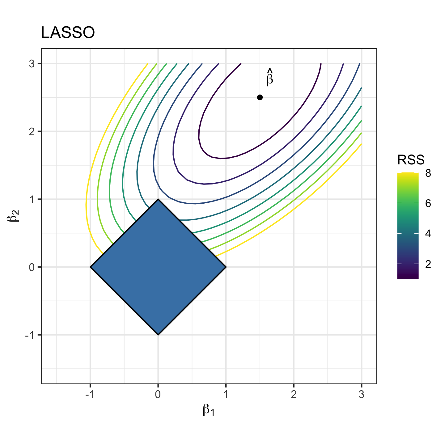
For LASSO, the solution to the optimization problem often lies on a vertex of the domain, which corresponds to a subspace where one or more parameters are \(0\).
Similarities:
Fast to estimate models (similar to Least Squares)
Shrink coefficients: Increasing bias but reducing variance and MSE
Differences:
LASSO performs variable selection simultaneously, Ridge does not.
LASSO generally outperforms Ridge when some coefficients are truly zero.
Ridge generally outperforms LASSO when all coefficients are truly non-zero.
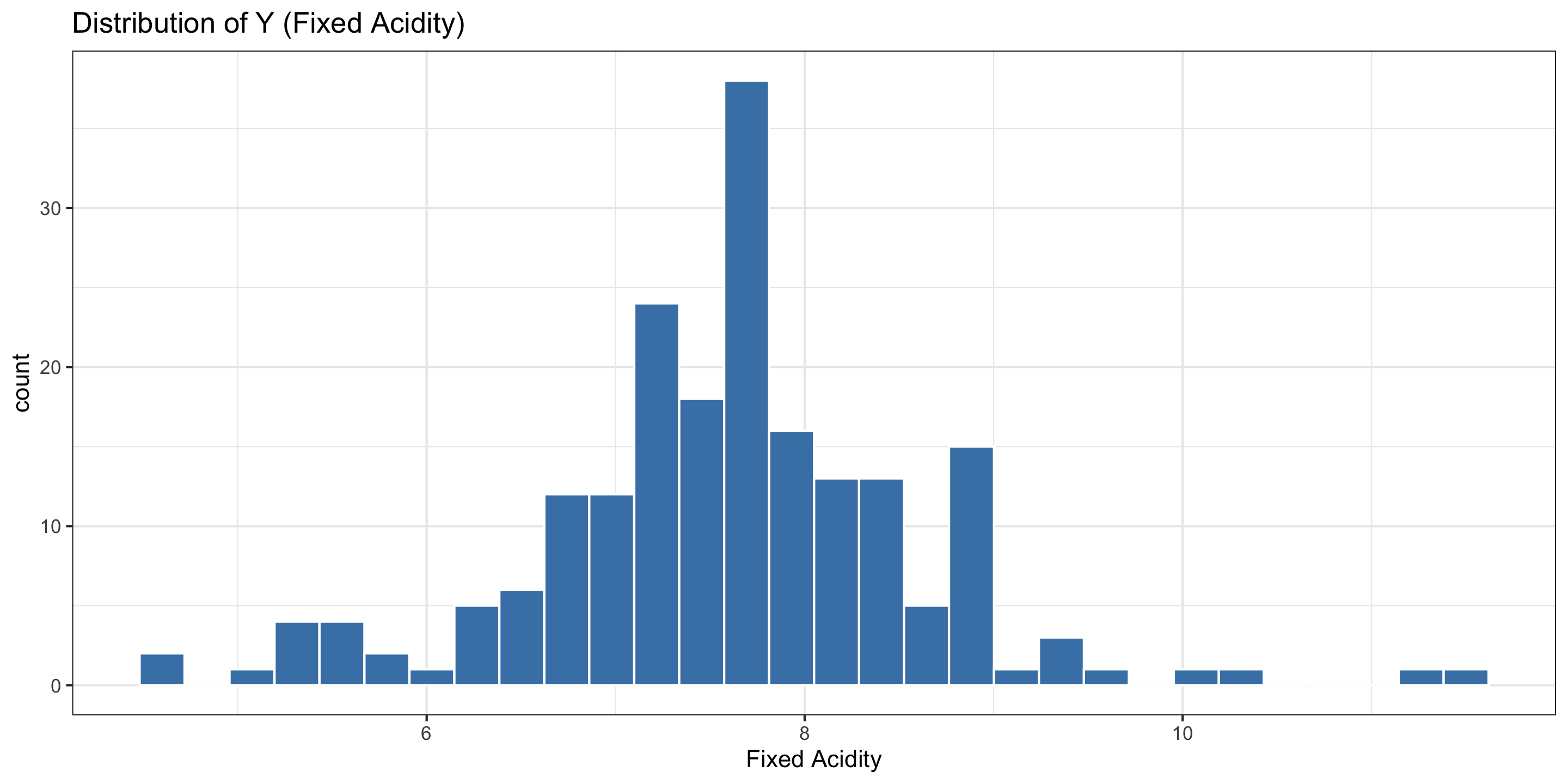
We study a “classic” dataset on red Vinho Verde wines grown in Northern Portugal.
\(n=200\) different wines
\(Y\)=Fixed Acidity
\(X\)=9 physical properties of the wine (e.g., residual sugar, pH, etc.) and average quality rating
# A tibble: 6 × 11
`fixed acidity` `volatile acidity` `citric acid` `residual sugar` chlorides
<dbl> <dbl> <dbl> <dbl> <dbl>
1 7.4 0.7 0 1.9 0.076
2 7.8 0.88 0 2.6 0.098
3 7.8 0.76 0.04 2.3 0.092
4 11.2 0.28 0.56 1.9 0.075
5 7.4 0.7 0 1.9 0.076
6 7.4 0.66 0 1.8 0.075
# ℹ 6 more variables: `free sulfur dioxide` <dbl>,
# `total sulfur dioxide` <dbl>, pH <dbl>, sulphates <dbl>, alcohol <dbl>,
# quality <dbl>

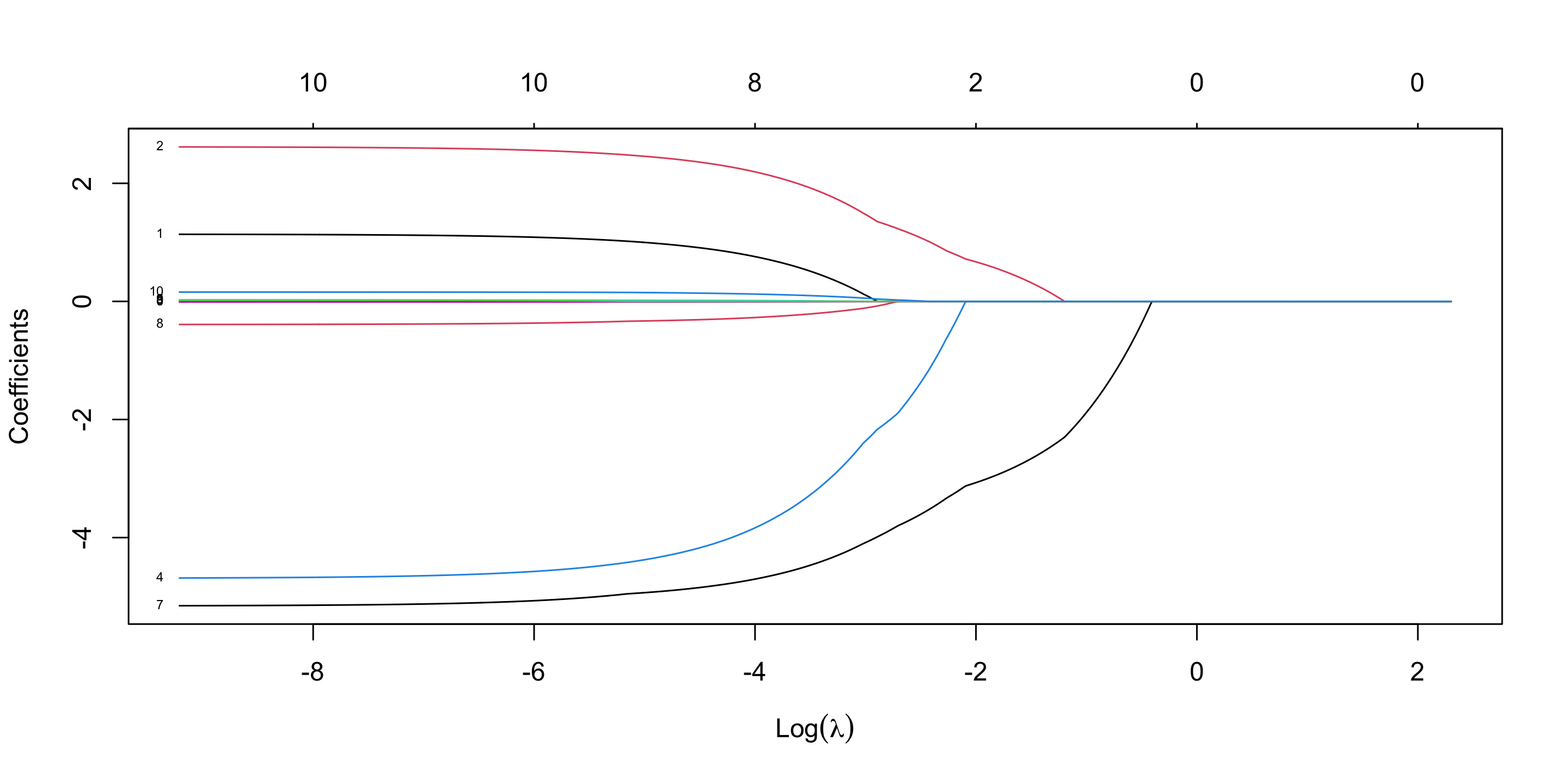
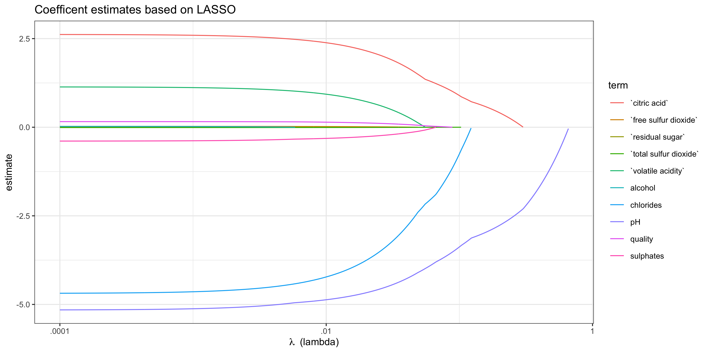
Q: Which coefficients will LASSO shrink to 0?
RExamine how LASSO coefficient estimates vary as \(\lambda\) changes:
tidied <- tidy(lasso_mod) %>% filter(term != "(Intercept)")
ggplot(tidied, aes(x = lambda, y = estimate, group = term, color = term)) +
geom_line() +
scale_x_log10(breaks = c(10^c(-4, -2, 0)),
labels = c(".0001", ".01", "1")) +
theme_bw(base_size = 10) +
labs(title = "Coefficent estimates based on LASSO",
x = expression(lambda ~ " (lambda)")) +
guides(color = guide_legend(ncol = 1))
To find the optimal tuning parameter, \(\lambda\), we again use Cross-Validation
set.seed(1010)
my_cv <- cv.glmnet(x,
y,
alpha = 1,
lambda = grid,
nfolds = 20)
best_L <- my_cv$lambda.min
reg_L <- my_cv$lambda.1se
tidied <- tidy(my_cv)
ggplot(tidied, aes(x = lambda, y = estimate)) +
geom_line(color = "red") +
scale_x_log10(breaks = c(10^c(-4, -2, 0)),
labels = c(".0001", ".01", "1")) +
theme_bw(base_size = 15) +
labs(x = expression(lambda), y = "Test MSE") +
geom_vline(xintercept = best_L, color = "goldenrod") +
geom_vline(xintercept = reg_L, color = "steelblue")
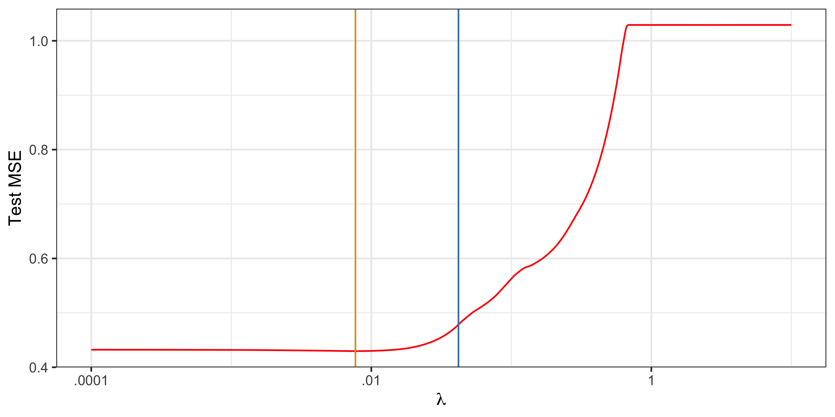
Gray vertical line is optimal \(\lambda\): Test MSE minimized at 0.4297.
(Ridge yields Test MSE of 0.4317)
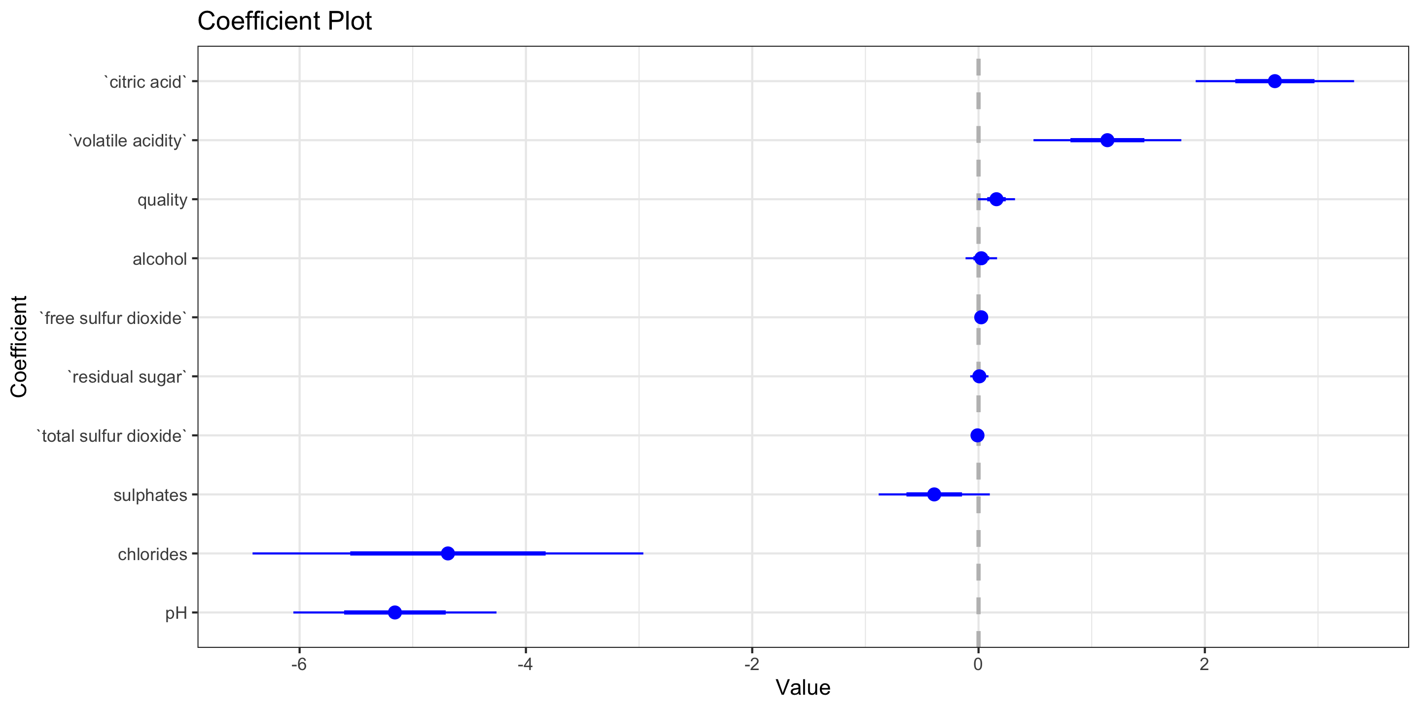
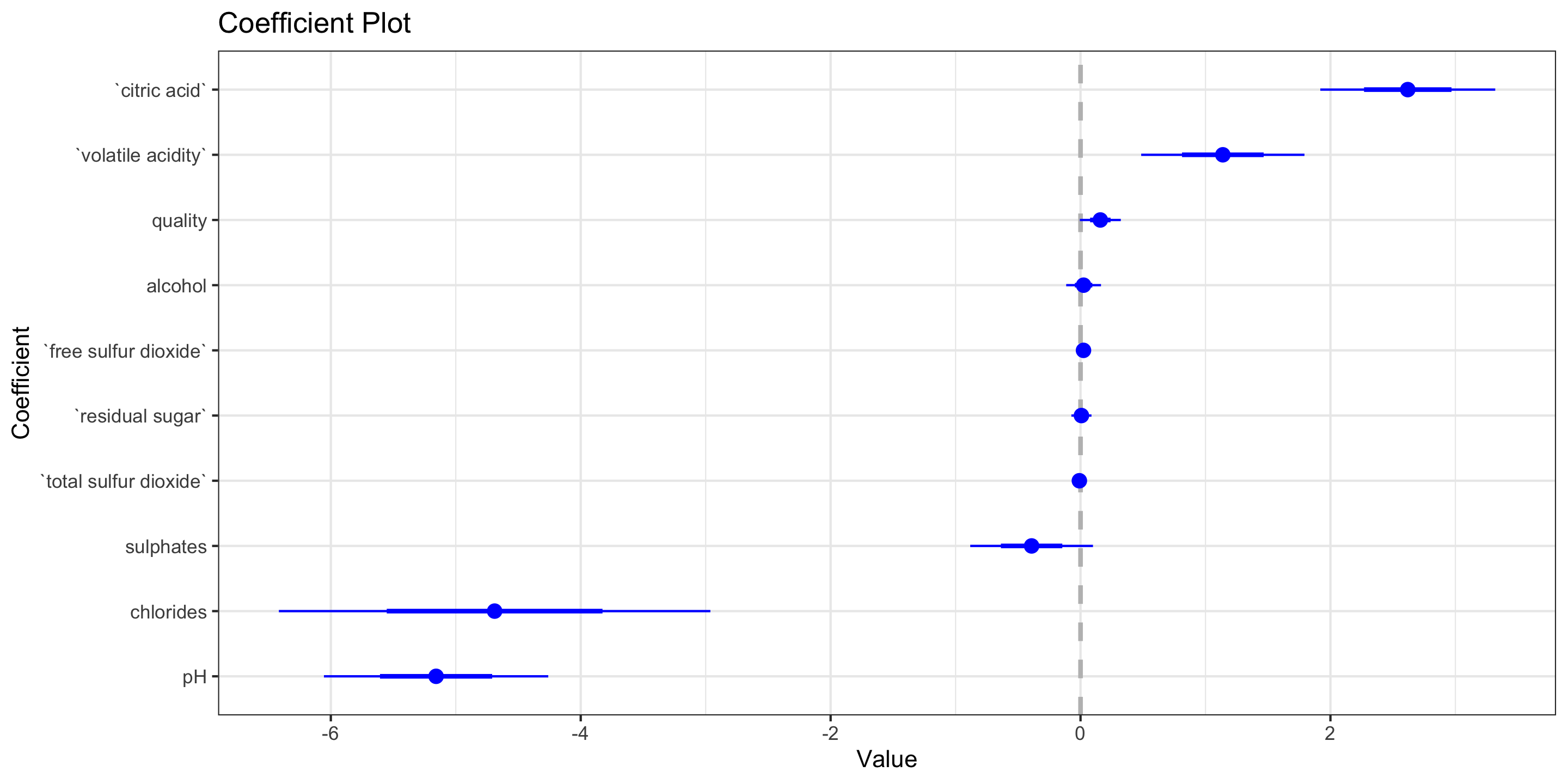
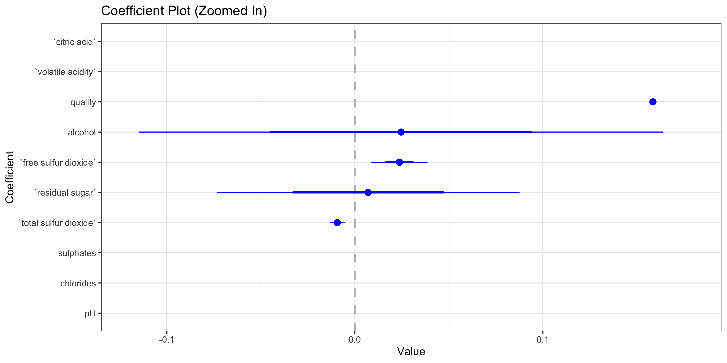
What features did the best \(\lambda\) select?
[1] "(Intercept)" "`volatile acidity`" "`citric acid`"
[4] "`residual sugar`" "chlorides" "`free sulfur dioxide`"
[7] "`total sulfur dioxide`" "pH" "sulphates"
[10] "quality"

LASSO removed only a high variance coefficient that was near 0.
Today, we learned about…
LASSO as a penalization and variable selection method
Similarities and differences with Ridge
Next time