
Penalized Regression: Ridge


Grayson White

Stat 243
Week 6 | Fall 2026

Goals for this week

Today:

  • Introduce penalization to improve MSE in regression models

  • Define and apply Ridge Regression in a case study

Next time:

  • Introduce LASSO as a penalization and variable selection method

  • Apply LASSO in a case study

Penalized Regression

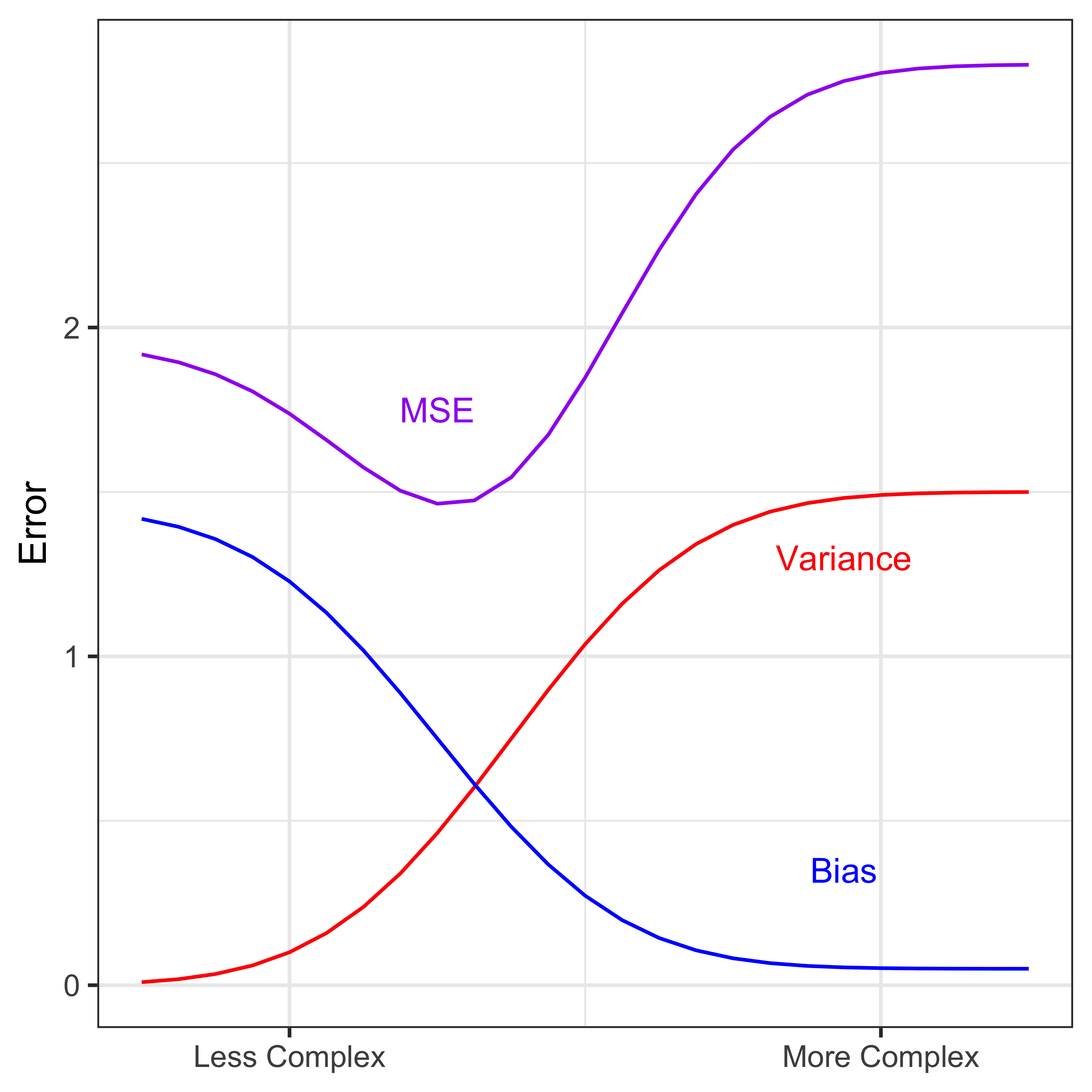
Recall: Bias-Variance Trade-Off

Bias-Variance Trade-off is useful when selecting among candidate models


Linear Regression:

  • Few predictors (less complex)
  • Many predictors (more complex)

Recall: Model Selection

Suppose we considered numerous “candidate” models, and picked one using cross-validation:

\[Y = \beta_0 + \beta_1X_1 + \beta_2X_2 + \epsilon,\qquad \epsilon\sim N(0,~\sigma^2)\]

Next, estimate coefficients using least-squares

\[\begin{aligned} \text{Find }& \ \hat\beta_0,\hat\beta_1,\hat\beta_2\ \text{ that minimizes }RSS\\ RSS&=\sum_{i=1}^n\Big(Y_i - (\hat\beta_0 + \hat\beta_1X_{1i} + \hat\beta_2X_{2i})\ \Big)^2 \end{aligned}\]

Remember: The model we chose minimized MSE among the candidate models: \[\text{MSE} = \text{Bias}^2 + \text{Variance}\]

Q: Could we further lower MSE, without changing the variables in our model?

A: Yes! We can change how we estimate the coefficients.

Penalization

This week, we’re focusing on two penalization methods for estimating regression coefficients.

  • Note: “Penalization”, “Regularization”, and “Shrinkage” are synonyms

General Premise:

  • “Shrink” magnitude of least-squares coefficients
  • This always increases bias \(\rightarrow\) bad!
  • Maybe it will decrease variance a lot \(\rightarrow\) good!

Overall Effect: Decrease MSE (hopefully!)

Toy Example

Suppose we have the following model: \[ Y = \beta_0 + \beta_1X_1 + \beta_2X_2 \]

Least Squares Regression Coefficients: \[\hat\beta_0 = 2, \ \ \hat\beta_1 = 3, \ \ \hat\beta_2 = 5\]

Two Models:

\[\begin{aligned} \text{Least Squares: }&Y = \hat\beta_0 \ + &\hat\beta_1X_1+\ \ \ & \ \ \ \ \hat\beta_2X_2 \\ \text{Shrunken Model: }&Y = \hat\beta_0 \ + &.98\hat\beta_1X_1+\ \ \ &0.95\hat\beta_2X_2 \\ \end{aligned}\]

Toy Example: Mathematical Explanation

\[\begin{aligned} \text{Least Squares: }&Y = 2 \ + &3X_1+\ \ \ & \ \ \ \ \ 5X_2 \\ \text{Shrunken Model: }&Y = 2 \ + &2.94X_1+\ \ \ &4.75X_2 \\ \end{aligned}\]

Shrunken Model has higher Bias than Least Squares – we modified the coefficients!

Shrunken Model has lower Variance than Least Squares

  • Recall: \(Var(cX) = c^2Var(X)\)
  • Intuition:

\[\text{Least Squares: }Var(3X_1)=9Var(X_1)\]

\[\text{Shrunken Model: }Var(2.94X_1)=8.64Var(X_1)\]

\[8.64Var(X_1) < 9Var(X_1)\]

Toy Example: Simulation Example

set.seed(100)
x1 <- runif(20, 0, 1)
x2 <- 2 - 2*x1 + rnorm(20, 0, .3)
e <- rnorm(20, 0, 1)
y <- 1 + x1 + 5*x2 + e
data <- data.frame(x1, x2, y)
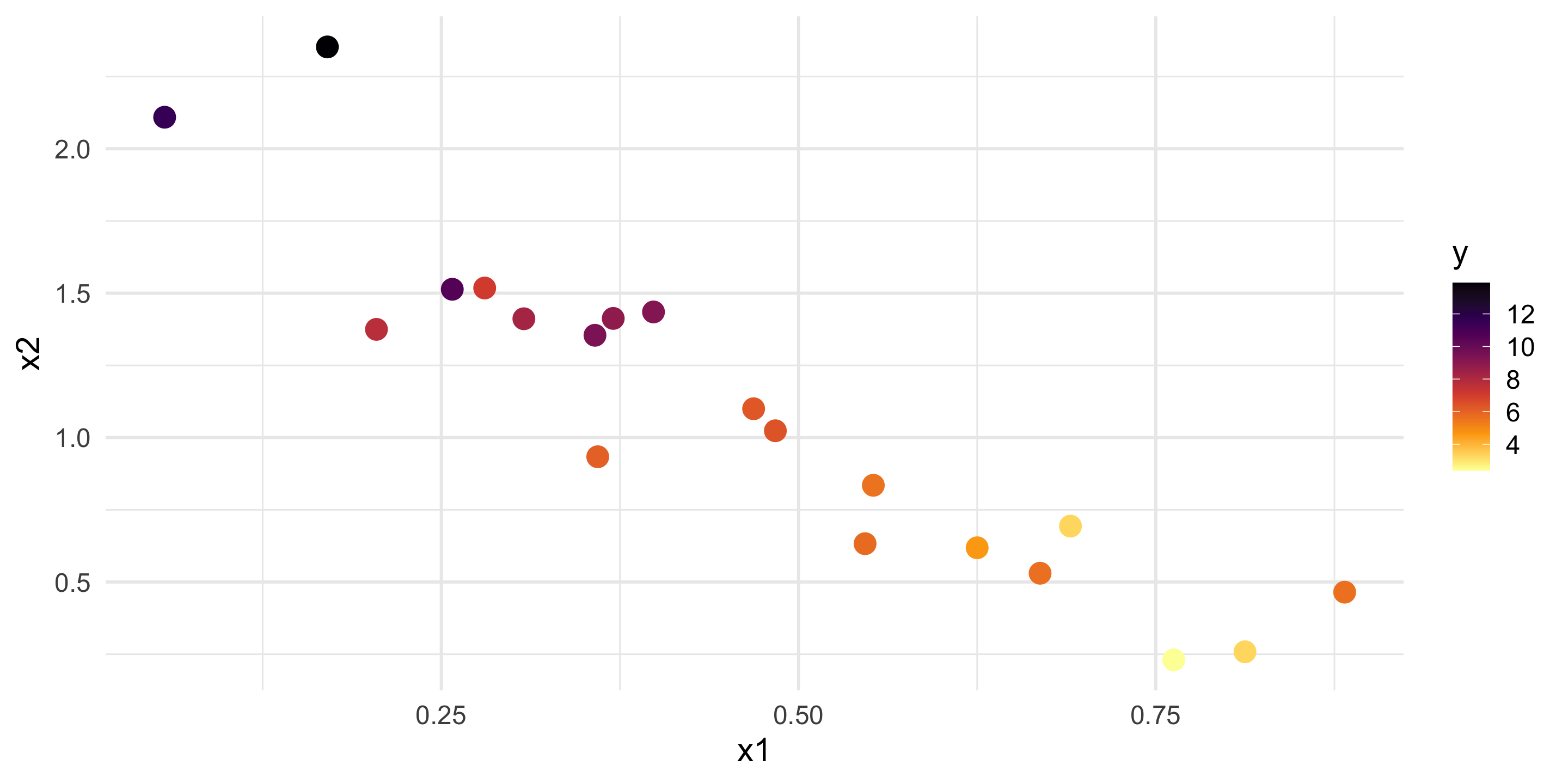
ggplot(data, aes(x = x1, y = x2, color = y)) + 
  geom_point(size = 4) + 
  theme_minimal(base_size = 15) +
  scale_color_viridis_c(option = "B", direction = -1)

We will:

  1. Split data into training and test sets
  2. Fit least squares model to the training data
  3. Make predictions on the test data using the “Least Squares” and “Shrunken Models”
  4. Compare MSE

Toy Example: Simulation Example

Step 1: Split data into training and test sets

set.seed(2)
train_indices <- sample(1:20,15)
train <- data[train_indices,]
test <- data[-train_indices,]

Step 2: Fit least squares model to the training data

least_squares <- lm(y ~ x1 + x2, data = train)
coef(least_squares)
(Intercept)          x1          x2 
  0.6764753   1.5186322   5.2849000 

Toy Example: Simulation Example

Step 3: Make predictions on the test data using the “Least Squares” and “Shrunken Models”

ypred_least_squares <- 0.676  + 1.519*test$x1 + 5.285*test$x2
ypred_shrunken_mod  <- 0.676  + 0.95*1.519*test$x1 + 0.98*5.285*test$x2
  • Could also use the predict() function for the least squares model.

Step 4: Compare MSE

MSE_LeastSquares <- mean( (ypred_least_squares-test$y)^2 )
MSE_ShrunkenMod  <- mean( (ypred_shrunken_mod -test$y)^2 )
c(MSE_LeastSquares, MSE_ShrunkenMod)
[1] 0.3202499 0.2834931

The shrunken model has lower MSE!

When Penalization Works

Consider situations where regression has high MSE:

  1. Predictors are strongly correlated (high variance)

  2. Many predictors relative to data size (high variance)

  3. Model form is non-linear (high bias)

To improve models in cases (1) and (2), we could “shrink” coefficients

  • Potentially big decreases in variance!

  • Bias might go up a bit, but maybe that’s okay.

  • Hopefully: MSE decreases overall.

Big Question: How do we actually “shrink” coefficients?

Ridge Regression

Ridge Regression

\[\text{Regression Model:} \ \ \ \ \ \ \ \ Y = \beta_0 + \beta_1X_1 + \dots + \beta_pX_p\]

Least Squares: Find \(\hat\beta\)s that minimize \[RSS=\sum_{i=1}^n\Big(Y_i - \underbrace{(\hat\beta_0 + \hat\beta_1X_{1i} + \dots + \hat\beta_pX_{pi})}_{\hat Y_i}\ \Big)^2\]

  • Goal of RSS: Make regression line “close to data”

Ridge Regression: Find \(\hat\beta\)s that minimize \[ \textrm{RSS} + \underbrace{\lambda\sum_{j = 1}^p \hat\beta_j^2}_\text{Ridge Penalty} \qquad \textrm{where } \lambda \geq 0 \text{ is a set \textbf{tuning parameter}} \]

Consider: Effects of the Tuning Parameter, \(\lambda\)

Ridge Regression: Find \(\hat\beta\)s that minimize \[ \textrm{RSS} + \underbrace{\lambda\sum_{j = 1}^p \hat\beta_j^2}_\text{Ridge Penalty} \]

  1. Imagine \(\lambda=0\). How do “Ridge” coefficients compare to “Least Squares” coefficients?
    • Ridge = Least Squares regression when \(\lambda=0\)
  2. What happens to \(\beta_1,\dots,\beta_p\) as \(\lambda\) gets bigger and bigger?
    • All \(\beta_1,\dots,\beta_p \rightarrow 0\) as \(\lambda\) grows.
  3. What happens to \(\beta_0\) (intercept) as \(\lambda\) gets bigger and bigger?
    • \(\beta_0 \to \bar{Y}\) as \(\lambda\) grows.
01:30

Note: Effect of Scale

Suppose that we find \(\hat{Y} = 1 + 5 X_1 + 20 X_2\) using Least Squares.

  • Recall: Coefficient Magnitude \(\neq\) Importance
  • Variables may have very different scales

Coefficients in Least-Squares regression and scale-equivalent

  • If we multiply a predictor (\(X_j\)) by \(2\), then the resulting coefficient (\(\hat{\beta}_j\)) would be multiplied by \(1/2\).

In Ridge Regression, coefficients can change depending on scale!

  • Variables with bigger scales are penalized more.

Software solves this problem:

  • Variables are “standardized”

  • Ridge Regression performed on standardized variables

  • Coefficients are re-scaled to the original scale.

Case Study: Molecule Solubility

Molecular Solubility

Data: Chemical properties for \(n\)=285 compounds

  • Response, \(Y\): log(Solubility). Solubility is how easily a compound dissolves in a solvent.

  • Predictors, \(X\): \(p=20\) chemical properties, such as “number of bromine atoms” or “molecular weight”.

Goal: Model solubility based on these 20 chemical descriptors.

Data preprocessing and EDA

library(AppliedPredictiveModeling)
data(solubility)

# Data preprocessing
solTest <- data.frame(solTestX, Solubility = solTestY)
solTrain <- data.frame(solTrainX, Solubility =  solTrainY)

solTest <- solTest %>% select(!starts_with("FP"))
solTrain <- solTrain %>% select(!starts_with("FP"))

# Considering a smaller training set (30% of original size)
set.seed(1)
solTrain <- solTrain %>% sample_frac(.3) 

# Plotting
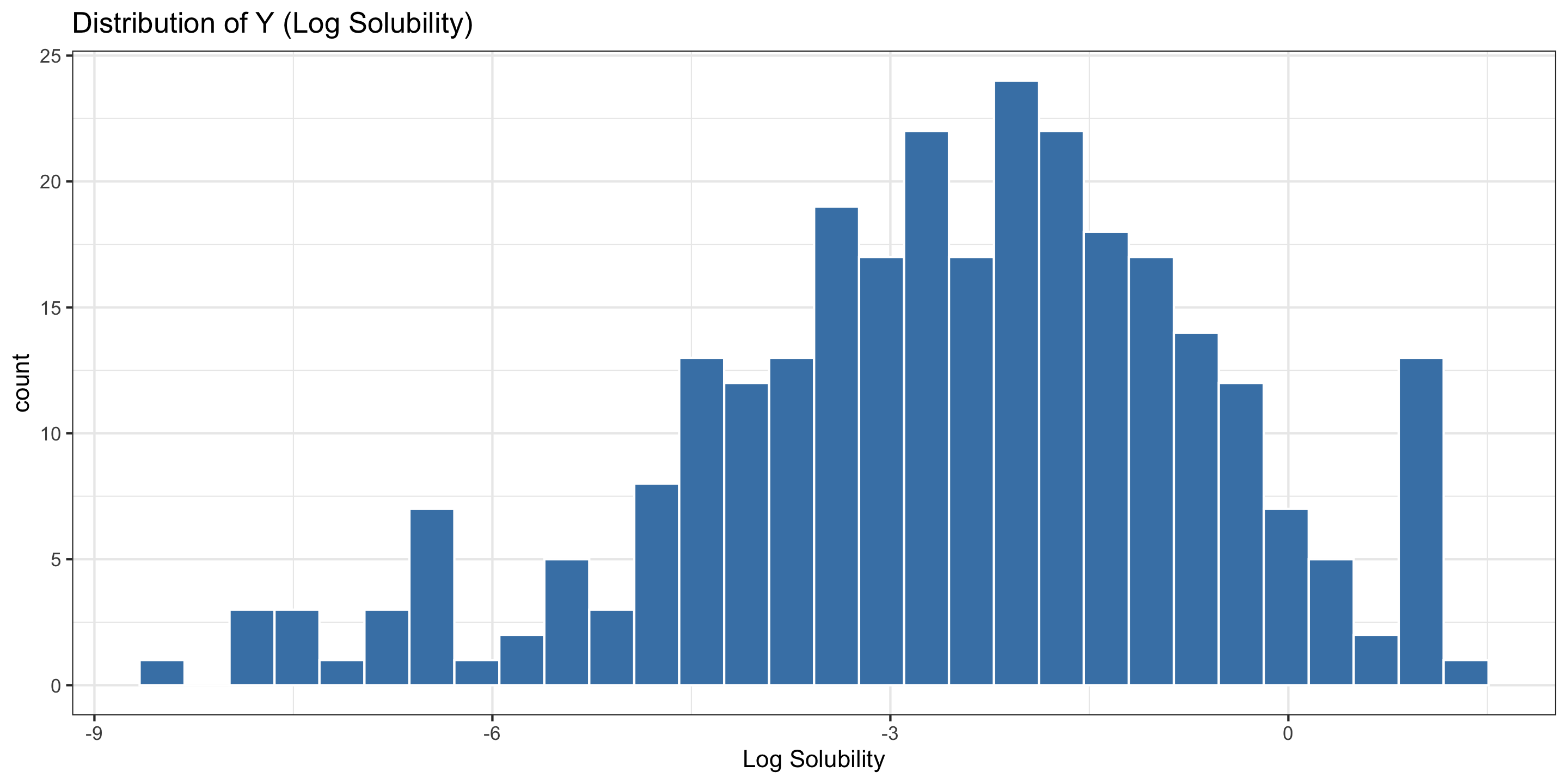
solTrain %>%
  ggplot(aes(x = Solubility)) +
  geom_histogram(color = "white",
                 fill = "steelblue") +
  labs(title = "Distribution of Y (Log Solubility)",
       x = "Log Solubility") +
  theme_bw()
Pairwise Scatterplots

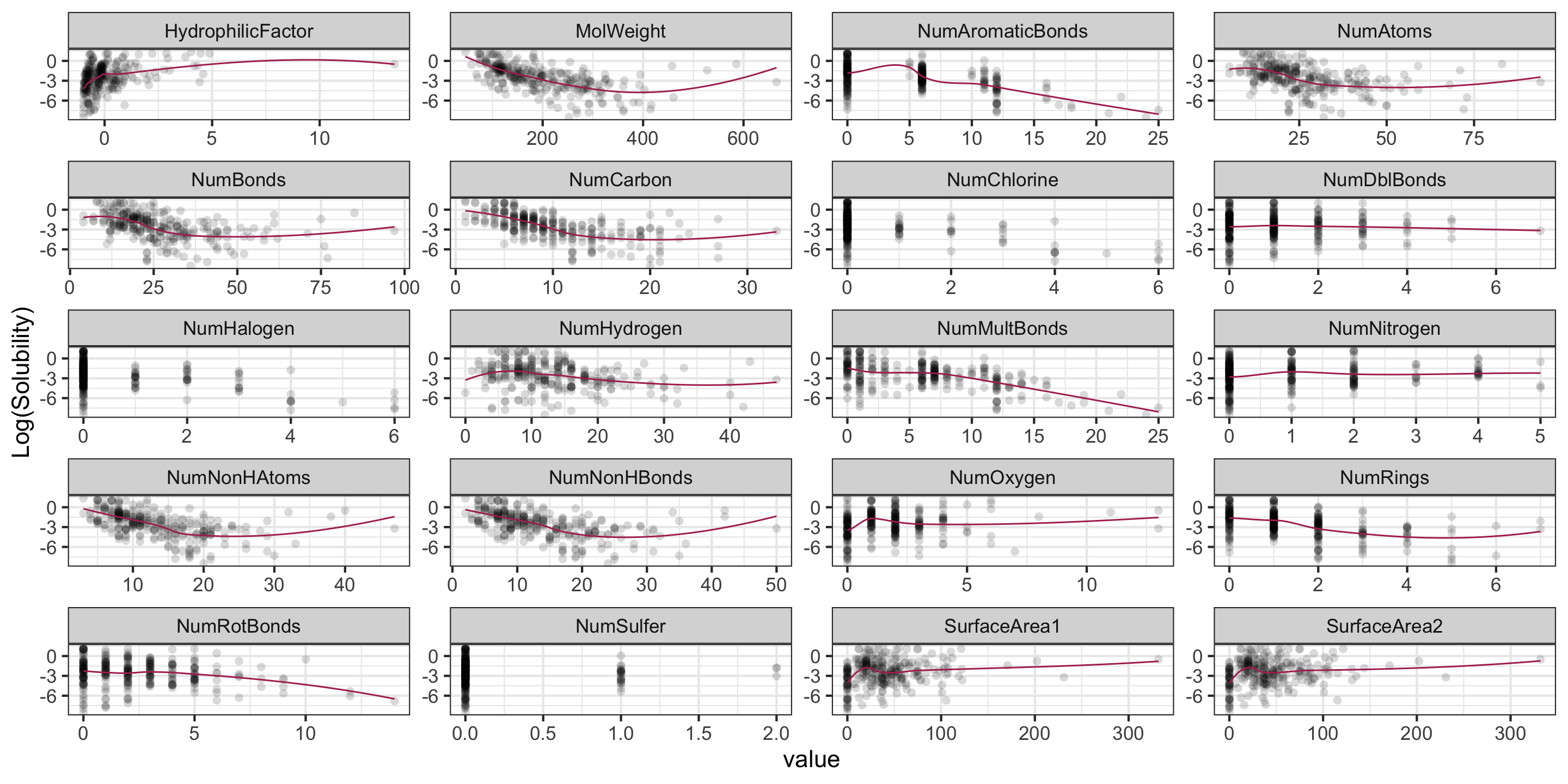
solTrain %>%
  pivot_longer(-Solubility, names_to = "var", values_to = "value") %>%
  ggplot(aes(x = value, y = Solubility)) +
  geom_point(alpha = .15, shape = 16) +
  geom_smooth(se = F, color = "maroon", linewidth = .35) +
  facet_wrap( ~ var, nrow = 5, scales = "free") +
  theme_bw() +
  labs(y = "Log(Solubility)")
Least Squares

Consider the least squares model fit to our data.

\[Y = \hat\beta_0 + \hat\beta_1X_1 + \dots + \hat\beta_{20}X_{20}\]

Suppose we have a test set to evaluate our model, consisting of (new) 316 compounds.

  • We compute test MSE:
full_mod <- lm(Solubility ~ ., data = solTrain)
preds <- predict(full_mod, solTest)
mean((solTest$Solubility - preds)^2)
[1] 0.9921199

Ridge Regression in R

Can we reduce the test MSE by “shrinking” the coefficients?

  • Let’s re-fit our model using several different values of \(\lambda\)…
# [,-1] removes the first column of this matrix, in this case,
# it is the intercept. We don't want to penalize the intercept!
x <- model.matrix(Solubility ~., data = solTrain)[,-1]
y <- solTrain$Solubility

grid <- 10^(seq(-5, 3, length = 100))

library(glmnet) # fits ridge regression models
ridge_mod <- glmnet(x = x,
                    y = y, 
                    # alpha = 0 specifies "ridge"
                    alpha = 0,
                    lambda = grid)

Ridge Coefficient Estimates, by \(\lambda\)
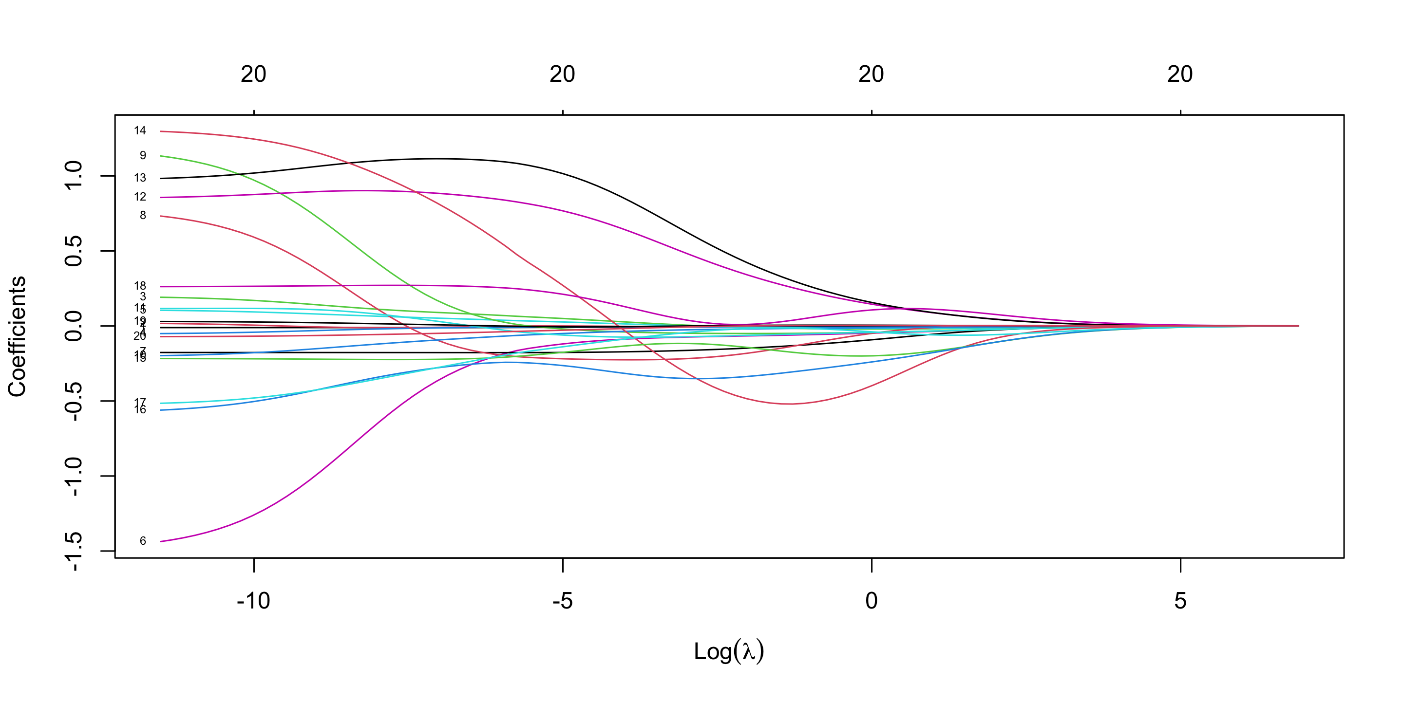
plot(ridge_mod, 
     sign.lambda = 1, 
     label = TRUE)

Q: What happens to coefficient size as \(\lambda\) changes?

Q: Why do some coefficients change sign as \(\lambda\) changes?

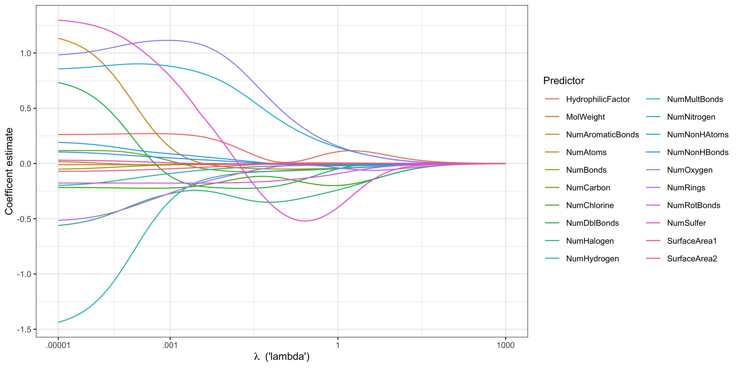
Ridge Coefficient Estimates, by \(\lambda\) with ggplot2

library(broom)
tidied <- tidy(ridge_mod) %>% 
  filter(term != "(Intercept)")
ggplot(tidied, aes(lambda, estimate, group = term, color = term)) +
  geom_line() +
  scale_x_log10(breaks = c(10^c(-5, -3, 0, 3)),
                labels = c(".00001", ".001", "1", "1000")) +
  theme_bw(base_size = 10) + 
  labs(y = "Coefficent estimate",
       color = "Predictor",
       x = expression(lambda~" ('lambda')")) +
  guides(color = guide_legend(ncol = 2))
How do we select \(\lambda\)?

Q: How do we find the best value of \(\lambda\)?

A: Cross-validation!

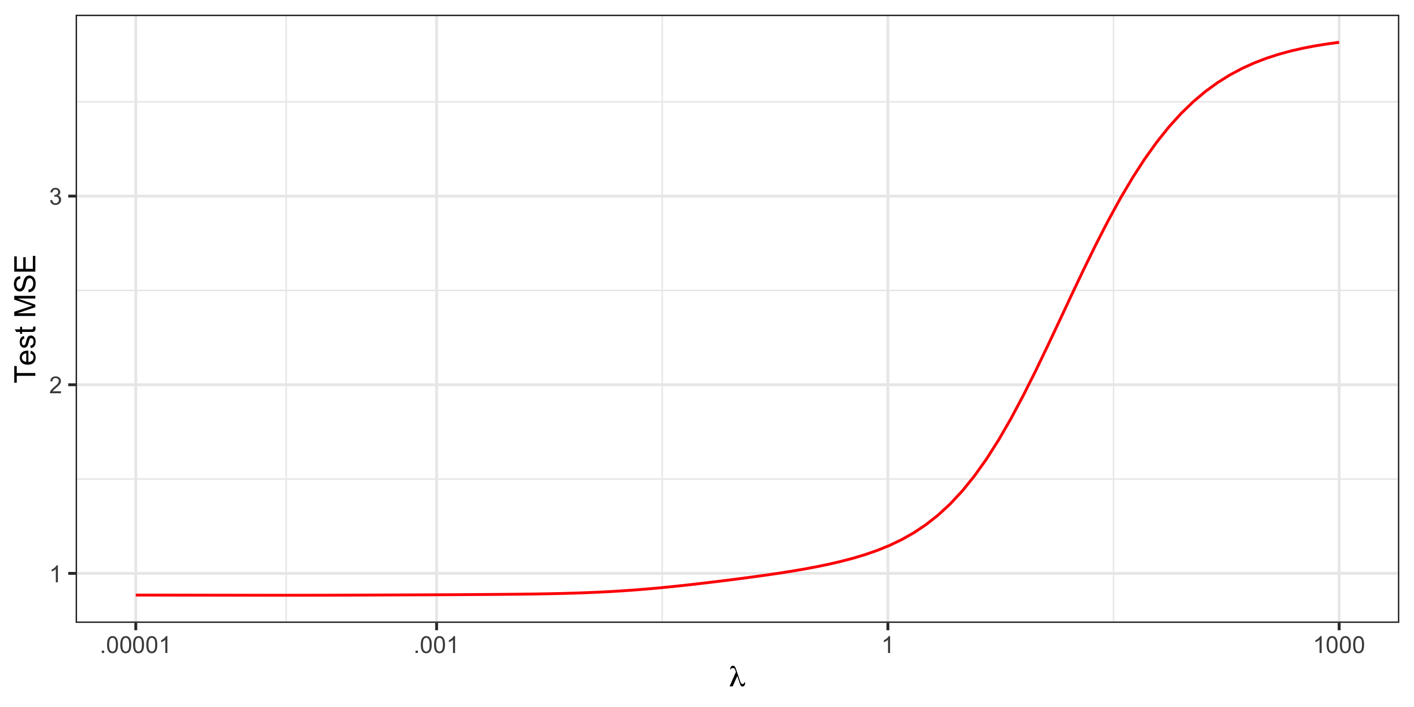
  • Compare test MSE between models fit using different values of \(\lambda\)

  • Select \(\lambda\) that minimizes the test MSE

  • This model represents an “optimal” relationship between bias and variance

Cross-Validation Estimate of Test MSE (10-fold CV)

set.seed(1010)
# Cross validation with glmnet
my_cv <- cv.glmnet(x = x,
                   y = y,
                   alpha = 0,
                   lambda = grid,
                   nfolds = 10)

# Plotting results
tidied <- tidy(my_cv)
ggplot(tidied, aes(x = lambda, y = estimate)) +
  geom_line(color = "red") +
  scale_x_log10(breaks = c(10^c(-5, -3, 0, 3)),
                labels = c(".00001", ".001", "1", "1000")) +
  theme_bw(base_size = 15) +
  labs(x = expression(lambda), y = "Test MSE")
Zooming In
tidied %>%
  filter(lambda <= 1e-03 & lambda >= 1e-5) %>%
  ggplot(aes(x = lambda, y = estimate)) +
  geom_line(color = "red") +
  scale_x_log10(breaks = c(10^c(-5:-3)),
                labels = c(".00001", ".0001", ".001")) +
  theme_bw(base_size = 15) +
  labs(x = expression(lambda), y = "Test MSE")

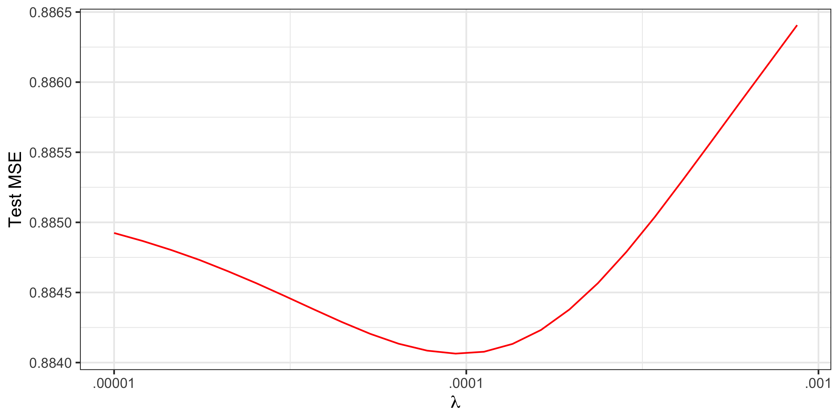
  • Test MSE is minimized at 0.8841 when \(\lambda = 0.0001\)

  • Recall: Original model had Test MSE = 0.992. Ridge Regression improved predictive performance!

Recap

Today, we learned about…

  • Shrinking coefficients to increase bias, but lower variance and MSE

  • Ridge Regression as one type of penalization

Next Time:

  • Introduce LASSO as a penalization and variable selection method

  • Apply LASSO in a case study