Cross Validation

Grayson White

Stat 243
Week 4 | Fall 2026

Goals for today (and next time)

Today:

Discuss model selection
Define and discuss resampling and cross-validation
Investigate methods of cross-validation (k-fold cv)
Implement CV in R

Friday:

Quiz 2 on Lab 2 material.
Lab 3 released.

Model Selection and Validation

Selecting a good model is central to this course

We can always select a model with tons of predictors, interactions, and non-linear terms.

\(R^2\) and training error are guaranteed to improve!
…we’re also likely to be overfitting.
p-values get larger, confidence intervals wider, interpretations harder, etc.

Selecting a “parsimonious” model usually lowers test MSE.

Principle of Parsimony: The simplest reasonable model is usually the best.

Selecting a good model is central to this course

Task: Choose model that retains only “important” predictors (i.e., \(\beta_k\neq0\))

Generally good practices:

If some variables are highly correlated, remove redundant ones
If \(R^2\) is low, try adding more variables
If adding a polynomial term (e.g., \(X^3\)), include lower terms too (e.g., \(X, \ X^2\))
If adding an interaction (e.g., \(X_1X_2\)), include individual terms too (e.g., \(X_1, \ X_2\))
Re-check diagnostics as you add/remove terms

Selecting a good model is central to this course

Task: Choose model that retains only “important” predictors (i.e., \(\beta_k\neq0\))

Generally bad practices:

Selecting a model based on p-values (e.g., forward/backward selection)
All downstream inferences are invalid; p-values lose all meaning
This is an example of “p-hacking,” which is a very big issue in applied research!

Q: Is there a more general way of selecting / validating a model?

A: Splitting the data into “training” and “test” sets!

Example: Fuel Economy

The FuelEconomy data (from the AppliedPredictiveModeling package) contains Fuel Efficiency (FE; in MPG) and other variables for 1107 cars and trucks from 2010

data taken from the http://fueleconomy.gov website

library(AppliedPredictiveModeling)
data(FuelEconomy)
glimpse(cars2010)

Rows: 1,107
Columns: 14
$ EngDispl            <dbl> 4.7, 4.7, 4.2, 4.2, 5.2, 5.2, 2.0, 6.0, 3.0, 3.0, …
$ NumCyl              <int> 8, 8, 8, 8, 10, 10, 4, 12, 6, 6, 6, 6, 16, 8, 8, 8…
$ Transmission        <fct> AM6, M6, M6, AM6, AM6, M6, S6, S6, S6, M6, S7, M6,…
$ FE                  <dbl> 28.0198, 25.6094, 26.8000, 25.0451, 24.8000, 23.90…
$ AirAspirationMethod <fct> NaturallyAspirated, NaturallyAspirated, NaturallyA…
$ NumGears            <int> 6, 6, 6, 6, 6, 6, 6, 6, 6, 6, 7, 6, 7, 6, 6, 6, 6,…
$ TransLockup         <dbl> 1, 1, 1, 1, 0, 0, 0, 0, 1, 0, 1, 0, 0, 0, 1, 0, 0,…
$ TransCreeperGear    <dbl> 0, 0, 0, 0, 0, 0, 0, 0, 0, 0, 0, 0, 0, 0, 0, 0, 0,…
$ DriveDesc           <fct> TwoWheelDriveRear, TwoWheelDriveRear, AllWheelDriv…
$ IntakeValvePerCyl   <int> 2, 2, 2, 2, 2, 2, 2, 2, 2, 2, 2, 2, 2, 1, 1, 1, 1,…
$ ExhaustValvesPerCyl <int> 2, 2, 2, 2, 2, 2, 2, 2, 2, 2, 2, 2, 2, 1, 1, 1, 1,…
$ CarlineClassDesc    <fct> 2Seaters, 2Seaters, 2Seaters, 2Seaters, 2Seaters, …
$ VarValveTiming      <dbl> 1, 1, 1, 1, 1, 1, 1, 1, 1, 1, 1, 1, 1, 0, 0, 0, 0,…
$ VarValveLift        <dbl> 0, 0, 0, 0, 0, 0, 0, 0, 1, 1, 0, 0, 0, 0, 0, 0, 0,…

Data Exploration

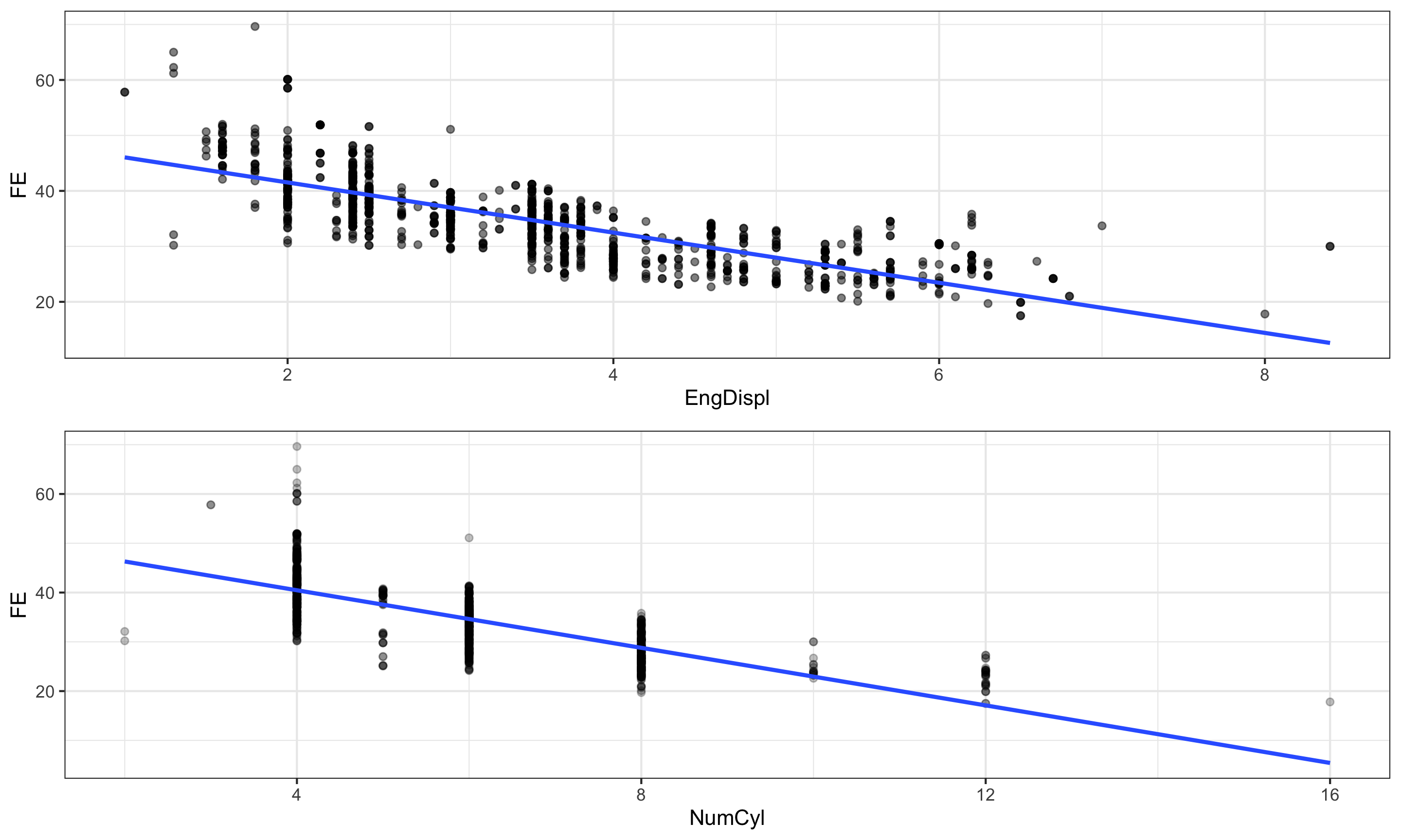
Let’s consider just numeric variables:

cars2010 %>%
  select_if(is.numeric) %>%
  cor(cars2010$FE)

                           [,1]
EngDispl            -0.78739383
NumCyl              -0.74021798
FE                   1.00000000
NumGears            -0.21128488
TransLockup         -0.27193887
TransCreeperGear    -0.06962168
IntakeValvePerCyl    0.28034403
ExhaustValvesPerCyl  0.33565285
VarValveTiming       0.12495278
VarValveLift         0.09621127

Variables highly correlated with FE:

Engine Displacement (EngDispl)
Number of Cylinders (NumCyl)

Collinearity

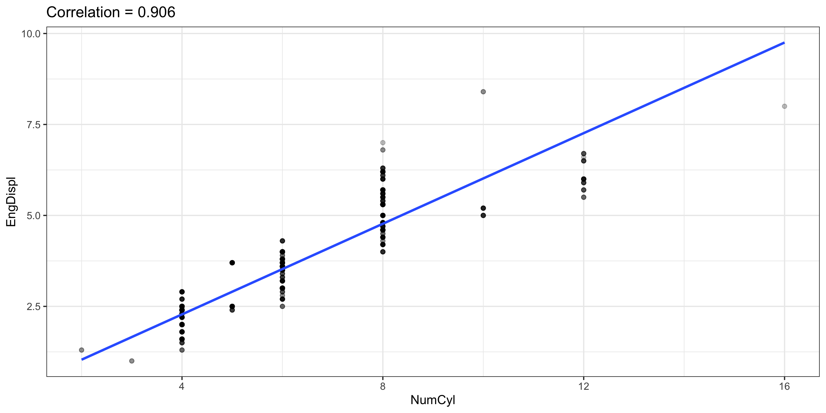
Do we want both EngDispl and NumCyl in our model for FE?

Each is strongly correlated with FE…

…thus, they might be highly collinear:

We now have a model selection problem: Which variables to include?

Training and Test Sets

Let’s create a 70-30 training-test split:

set.seed(1)
train_index <- sample(1:nrow(cars2010), 0.7*nrow(cars2010))
cars_train <- cars2010[train_index,]
cars_test <- cars2010[-train_index,]

We will fit two models:

fullmod includes all quantitative predictors
smallmod will exclude NumCyl, NumGears, IntakeValvePerCy, and VarValveLift

Let’s train!

Training: Fit each model to the training data

fullmod <- lm(FE ~ EngDispl + NumCyl + NumGears + TransLockup + 
                TransCreeperGear + IntakeValvePerCyl + ExhaustValvesPerCyl +
                VarValveTiming + VarValveLift,
              data = cars_train)
smallmod <- lm(FE ~ EngDispl + TransLockup + TransCreeperGear +
              ExhaustValvesPerCyl + VarValveTiming,
              data = cars_train)
round(c(summary(fullmod)$r.sq, summary(smallmod)$r.sq), 3)

[1] 0.628 0.624

fullmod has a slightly higher \(R^2\), but is it really better?

And now we test!

Testing: Calculate MSE on the test set

fullmod_preds <- predict(fullmod, cars_test)
fullmod_mse <- mean( (cars_test$FE - fullmod_preds)^2)
fullmod_mse

[1] 18.45154

smallmod_preds <- predict(smallmod, cars_test)
smallmod_mse <- mean( (cars_test$FE - smallmod_preds)^2)
smallmod_mse

[1] 18.7632

smallmod has slightly higher test MSE than fullmod!

Could this be a fluke of our randomly-split test set?

Problems with Test Sets

Q: What are some problems with this simple Training / Test approach?

If full dataset is small, splitting into training/test further restricts sample size
- Both training and test performance may have high variance.

A single randomly-split training set may be unusual \(\to\) Bias in model validation

A single randomly-split test set doesn’t give good estimate for amount of error.

How to Improve the Training/Testing Procedure:

Cross-Validation (CV):
- Resample many samples from training data and refit model in each sample.
- Assess model accuracy by “cross-validating” to many test set

Resampling and CV

\(k\)-fold Cross Validation (CV)

\(k\)-fold CV: Start by randomly partitioning data into \(k\) sets, or folds, of size \(n/k\). Then,

Choose one subset of size \(n/k\) as the validation set
Use the remaining \(k-1\) subsets as the training set to build the model
Calculate error rate (e.g., MSE) on the validation set

Repeat Steps 1-3 for each validation set
Average the error rate computed among the \(k\) validation sets

\(k\)-fold Cross Validation (CV)

The cross-validation estimate \(CV_{(k)}\) for average test MSE is: \[ CV_{(k)} = \frac{1}{k} \sum_{i =1}^k \textrm{MSE}_i \] where \(\textrm{MSE}_i\) is test MSE when the \(i\)th set, or fold, is used as validation set.

Because the partitioning into folds is random, \(CV_{(k)}\) still has some variability.

But less than just using a single validation set!
To reduce variability further, \(k\)-fold CV can be performed multiple times, and the results of \(CV_{(k)}\) themselves averaged.

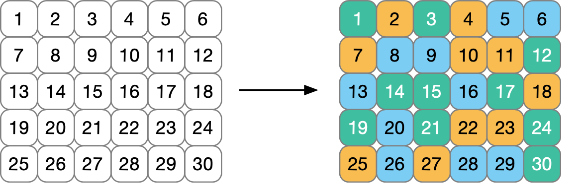
Ex: 3-fold CV

Consider 30 training observations below. Colors indicate a random fold allocation.

Ex: 3-fold CV

Each iteration uses 2 of the folds to build a model, and the remaining fold to assess performance.

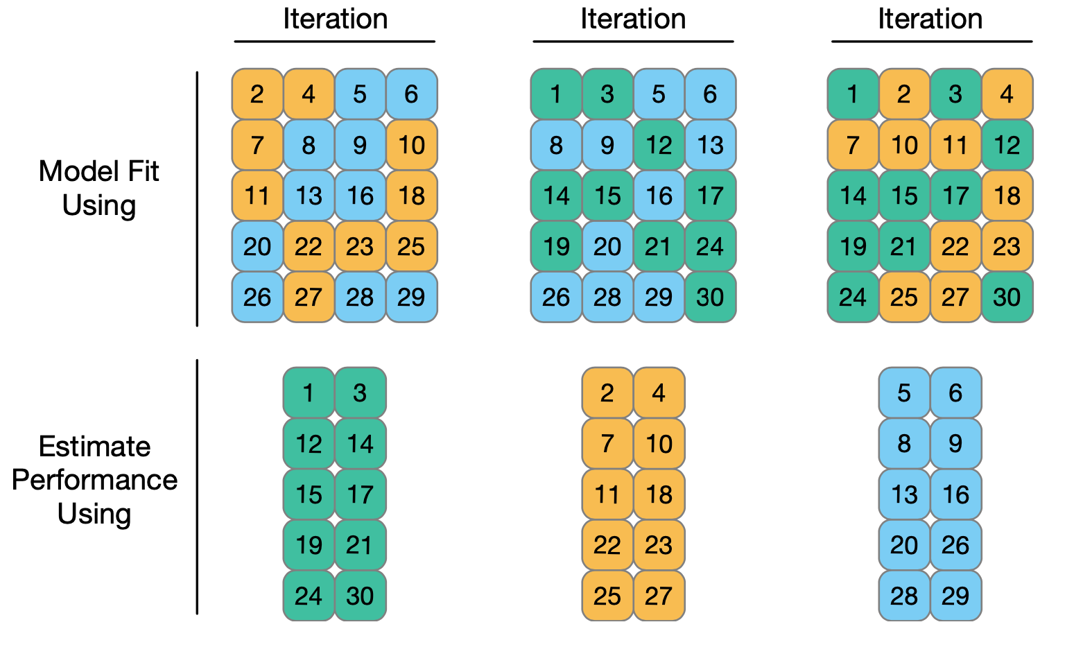
Overall performance is obtained by averaging across iterations.

CV in R: the `vfold_cv` function

We’ll use the vfold_cv function in rsample to perform cross-validation.

set.seed(927)
library(rsample)
folds_cars <- vfold_cv(cars2010, v = 10)

This code splits the data into 10 (nearly) equal folds and stores results as a resample object with 2 parts:

id, a vector with fold identifiers (i.e “Fold01”, “Fold02”, … )

folds_cars$id

 [1] "Fold01" "Fold02" "Fold03" "Fold04" "Fold05" "Fold06" "Fold07" "Fold08"
 [9] "Fold09" "Fold10"

splits, an R list whose elements correspond to each split of the data into \(k-1\) training and \(1\) validation sets

CV in R: the `vfold_cv` function

Previous Code:

folds_cars <- vfold_cv(cars2010, v = 10)

Get Training Set for a fold: apply analysis to one of the Splits elements.

folds_cars$splits[[1]] %>% analysis() # gets first "training set"
folds_cars$splits[[2]] %>% analysis() # gets second "training set"

Get Corresponding Test Set: apply assessment to the same Splits element

folds_cars$splits[[1]] %>% assessment() # observations NOT in first "training set"
folds_cars$splits[[2]] %>% assessment() # observations NOT in second "training set"

Goal: use cross-validation to assess which model is “best”

Steps:

Obtain training set
Fit linear model
Predict on assessment/validation data
Assess accuracy

rsample package did all the splitting for us (step 1)!

But no model fitting or computing MSE (steps 2 - 4).
How to do steps 2 - 4?

Fit the all the models!

We could do steps 2 -4 “by hand”, e.g.,

full_train_1 <- lm(FE ~ EngDispl + NumCyl + NumGears + TransLockup + 
                TransCreeperGear + IntakeValvePerCyl + ExhaustValvesPerCyl +
                VarValveTiming + VarValveLift,
              data = folds_cars$splits[[1]] %>% analysis())

small_train_1 <- lm(FE ~ EngDispl + TransLockup + TransCreeperGear +
              ExhaustValvesPerCyl + VarValveTiming,
              data = folds_cars$splits[[1]] %>% analysis())

full_pred_1 <- predict(full_train_1, newdata = folds_cars$splits[[1]] %>% assessment())

small_pred_1 <- predict(small_train_1, newdata = folds_cars$splits[[1]] %>% assessment())

RMSE_full_1 <- sqrt(mean( (full_pred_1 - folds_cars$splits[[1]] %>% assessment() %>% pull(FE))^2))

RMSE_small_1 <- sqrt(mean( (small_pred_1 - folds_cars$splits[[1]] %>% assessment() %>% pull(FE))^2))

RMSE_full_1

[1] 3.959213

RMSE_small_1

[1] 3.959354

Need to loop over all splits (1, 2, 3, …, 10).
Could write this into a function() or a for() loop and do it ourselves…

For loop approach

n_folds <- 10
RMSE_full <- list()
RMSE_small <- list()
for (i in 1:n_folds) {
  full_train_i <- lm(
    FE ~ EngDispl + NumCyl + NumGears + TransLockup +
      TransCreeperGear + IntakeValvePerCyl + ExhaustValvesPerCyl +
      VarValveTiming + VarValveLift,
    data = folds_cars$splits[[i]] %>% analysis()
  )
  
  small_train_i <- lm(
    FE ~ EngDispl + TransLockup + TransCreeperGear +
      ExhaustValvesPerCyl + VarValveTiming,
    data = folds_cars$splits[[i]] %>% analysis()
  )
  
  full_pred_i <- predict(full_train_i, newdata = folds_cars$splits[[i]] %>% assessment())
  
  small_pred_i <- predict(small_train_i, newdata = folds_cars$splits[[i]] %>% assessment())
  
  RMSE_full[[i]] <- sqrt(mean((full_pred_i - folds_cars$splits[[i]] %>% assessment() %>% pull(FE))^2))
  
  RMSE_small[[i]] <- sqrt(mean((small_pred_i - folds_cars$splits[[i]] %>% assessment() %>% pull(FE))^2))
}

mean(unlist(RMSE_full))

[1] 4.508613

mean(unlist(RMSE_small))

[1] 4.520042

Not super nice code…
We can use the tidymodels!

`tidymodels`

The tidymodels are a collection of packages built for predictive modeling that maintain consistent syntax across model types.
- e.g., fitting a linear regression model and a tree-based regression model (which we’ll learn about after Fall Break) require almost identical code!
Lots of really thoughtful built-in functions for predictive modeling.
Developed and maintained by the folks at Posit, who created RStudio and the tidyverse.
Simon Couch ’21 worked extensively on the tidymodels after graduating from Reed, although now he works on a different team at Posit.

Fitting models with the `tidymodels`

Consider our smallmod.

smallmod <- lm(
  FE ~ EngDispl + TransLockup + TransCreeperGear + 
  ExhaustValvesPerCyl + VarValveTiming,
  data = cars_train
)

smallmod


Call:
lm(formula = FE ~ EngDispl + TransLockup + TransCreeperGear + 
    ExhaustValvesPerCyl + VarValveTiming, data = cars_train)

Coefficients:
        (Intercept)             EngDispl          TransLockup  
            53.5896              -4.5647              -0.8766  
   TransCreeperGear  ExhaustValvesPerCyl       VarValveTiming  
            -1.5806              -1.7615               1.2568

With the tidymodels:

library(tidymodels)

smallmod_tidy <- linear_reg() %>%   
  set_engine("lm")  %>%          
  fit(FE ~ EngDispl + TransLockup + TransCreeperGear +
      ExhaustValvesPerCyl + VarValveTiming, 
      data = cars_train) 

smallmod_tidy

parsnip model object


Call:
stats::lm(formula = FE ~ EngDispl + TransLockup + TransCreeperGear + 
    ExhaustValvesPerCyl + VarValveTiming, data = data)

Coefficients:
        (Intercept)             EngDispl          TransLockup  
            53.5896              -4.5647              -0.8766  
   TransCreeperGear  ExhaustValvesPerCyl       VarValveTiming  
            -1.5806              -1.7615               1.2568

Fitting (many) models with the `tidymodels`

Consider our smallmod:

smallmod <- lm(FE ~ EngDispl + TransLockup + TransCreeperGear +
              ExhaustValvesPerCyl + VarValveTiming,
              data = cars_train)

With the tidymodels, we can specify this model form to be fit on many different datasets:

# loads the tidymodels
library(tidymodels)

# specifies we'd like to do linear regression with the lm() function
lm_spec <- linear_reg() %>%   
  set_engine("lm")            

# creates a "workflow" to be used on many datasets
# NOTICE: no data is supplied
smallmod_wf <- workflow() %>%
  add_model(lm_spec) %>%
  add_formula(FE ~ EngDispl + TransLockup + TransCreeperGear +
              ExhaustValvesPerCyl + VarValveTiming)

Get Results

fit_resamples() fits the workflow on each training set and evaluates it on the matching assessment set.

smallmod_res <- fit_resamples(
  smallmod_wf,
  resamples = folds_cars,
  metrics = metric_set(rmse)
)

collect_metrics() collects the metrics calculated on each test set.

collect_metrics(smallmod_res, summarize = FALSE)

# A tibble: 10 × 5
   id     .metric .estimator .estimate .config        
   <chr>  <chr>   <chr>          <dbl> <chr>          
 1 Fold01 rmse    standard        3.96 pre0_mod0_post0
 2 Fold02 rmse    standard        4.04 pre0_mod0_post0
 3 Fold03 rmse    standard        4.86 pre0_mod0_post0
 4 Fold04 rmse    standard        5.03 pre0_mod0_post0
 5 Fold05 rmse    standard        4.50 pre0_mod0_post0
 6 Fold06 rmse    standard        4.18 pre0_mod0_post0
 7 Fold07 rmse    standard        4.98 pre0_mod0_post0
 8 Fold08 rmse    standard        4.31 pre0_mod0_post0
 9 Fold09 rmse    standard        4.85 pre0_mod0_post0
10 Fold10 rmse    standard        4.50 pre0_mod0_post0

Get Results

fit_resamples() fits the workflow on each training set and evaluates it on the matching assessment set.

smallmod_res <- fit_resamples(
  smallmod_wf,
  resamples = folds_cars,
  metrics = metric_set(rmse)
)

collect_metrics() collects the metrics calculated on each test set.

collect_metrics(smallmod_res)

# A tibble: 1 × 6
  .metric .estimator  mean     n std_err .config        
  <chr>   <chr>      <dbl> <int>   <dbl> <chr>          
1 rmse    standard    4.52    10   0.124 pre0_mod0_post0

Comparing Models

Now, we can run the same code for our fullmod:

fullmod_wf <- workflow() %>%
  add_model(lm_spec) %>%
  add_formula(FE ~ EngDispl + NumCyl + NumGears + TransLockup + 
                TransCreeperGear + IntakeValvePerCyl + ExhaustValvesPerCyl +
                VarValveTiming + VarValveLift) 

fullmod_res <- fit_resamples(
  fullmod_wf,
  resamples = folds_cars,
  metrics = metric_set(rmse)
)

collect_metrics(fullmod_res)

# A tibble: 1 × 6
  .metric .estimator  mean     n std_err .config        
  <chr>   <chr>      <dbl> <int>   <dbl> <chr>          
1 rmse    standard    4.51    10   0.120 pre0_mod0_post0

Note that we are using the same lm_spec as before.

Comparing Models

Which model is best?

collect_metrics(fullmod_res)

# A tibble: 1 × 6
  .metric .estimator  mean     n std_err .config        
  <chr>   <chr>      <dbl> <int>   <dbl> <chr>          
1 rmse    standard    4.51    10   0.120 pre0_mod0_post0

collect_metrics(smallmod_res)

# A tibble: 1 × 6
  .metric .estimator  mean     n std_err .config        
  <chr>   <chr>      <dbl> <int>   <dbl> <chr>          
1 rmse    standard    4.52    10   0.124 pre0_mod0_post0

How to choose the number of folds, \(k\)

Selecting the Number of Folds, \(k\)

What’s the smallest value \(k\) can be in \(k\)-fold CV? Largest?
- A: \(K\in\{2,3,\dots,n\}\)
What are some pros and cons of small \(k\)?
- Pro: Easier computation (fewer models to train), but…
- Con: Training data is small: doesn’t reflect true size of training data
What are some pros and cons of large \(k\)?
- Con: Harder computation (many models to train), but…
- Pro: Training data is large: reflect true size of training data

Selecting the Number of Folds, \(k\)

\(k = 10\) is a common ‘rule of thumb’. But choosing \(k\) depends on your data and context!!

If \(n\) is small, \(k = 10+\) is generally a good choice,
If \(n\) is large and computation time is long, \(k = 5\) typically does fine.

Next time:

Quiz on Lab 2 content.
Lab 3 released.

Goals for today (and next time)

Model Selection and Validation

Selecting a good model is central to this course

Selecting a good model is central to this course

Selecting a good model is central to this course

Example: Fuel Economy

Data Exploration

Collinearity

Training and Test Sets

Let’s train!

And now we test!

Problems with Test Sets

Resampling and CV

\(k\)-fold Cross Validation (CV)

\(k\)-fold Cross Validation (CV)

Ex: 3-fold CV

Ex: 3-fold CV

CV in R: the vfold_cv function

CV in R: the vfold_cv function

Goal: use cross-validation to assess which model is “best”

Fit the all the models!

Fit the all the models!

For loop approach

tidymodels

Fitting models with the tidymodels

Fitting (many) models with the tidymodels

Get Results

Get Results

Comparing Models

Comparing Models

How to choose the number of folds, \(k\)

Selecting the Number of Folds, \(k\)

Selecting the Number of Folds, \(k\)

Next time:

CV in R: the `vfold_cv` function

CV in R: the `vfold_cv` function

`tidymodels`

Fitting models with the `tidymodels`

Fitting (many) models with the `tidymodels`