Linear Regression III


Grayson White

Stat 243
Week 3 | Fall 2026

Goals for this week (and next time)

Today:

  • Inference for regression
  • Categorical predictors
  • Multiple linear regression

Next time:

  • Quiz on Lab 1 (20 mins)
  • Linear regression extensions (30 mins)
  • Lab 2 released

Inference for Linear Models

Statistical Inference

  • Goal: Use statistics calculated from data to make estimates about unknown parameters

  • Parameters: \(\beta_0\), \(\beta_1\)

  • Statistics: \(\hat{\beta}_0\), \(\hat{\beta}_1\)

  • Tools: confidence intervals, hypothesis tests

  • The Problems: Our model will change if built using a different random sample. So in addition to estimates, we need to know about variability

The Confidence Interval

  • Confidence Intervals give estimates and express an amount of uncertainty we have about those estimates
  • A \(C\)-level confidence interval for a parameter \(\theta\) using the statistic \(\hat{\theta}\) takes the form

\[ \hat{\theta} \pm t^*_C \cdot \widehat{\mathrm{SE}}(\hat{\theta}) \]

  • The value \(t^*_C\) is the \(1 - (1-C)/2\) quantile for the sampling distribution of \(\hat{\theta}\)
    • i.e. if \(\hat{\theta}\) is approximately Normally distributed and \(C = .95\), then \(t^*_C \approx 2\).
  • The value \(\widehat{\mathrm{SE}}(\hat{\theta})\) is the estimated standard error of \(\hat{\theta}\), or the estimated standard deviation of the sampling distribution

Common Regression Assumptions

In order to use simple linear regression for inference, we require the LINE assumptions.

  1. Linearity: The relationship between explanatory and response variables must be approximately linear

  2. Independence: The observations should be independent of one another.

  3. Normality: The distribution of residuals should be approximately bell-shaped, unimodal, symmetric, and centered at 0 at every “slice” of the explanatory variable

  4. Equal Variability: Variance of residuals should be roughly constant across data set. Also called “homoscedasticity”. Models that violate this assumption are sometimes called “heteroscedastic”

If one or more of these conditions do not hold, our predictions may not be accurate and we should be skeptical of inferential claims.

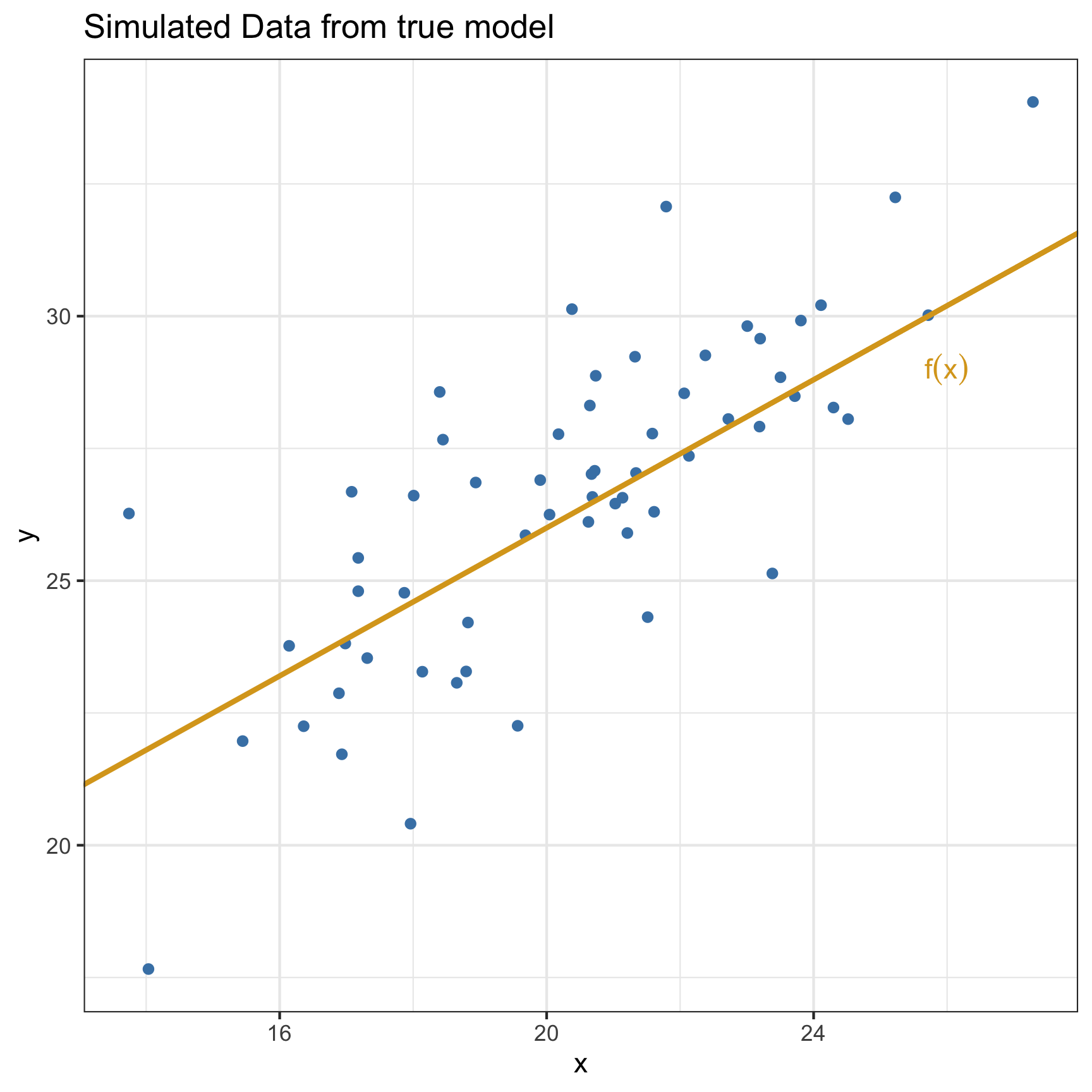
The Sampling Distribution of \(\hat{\beta}_1\)

Assume the following true model: \[ f(x) = 12 + 0.7 x; \quad \epsilon \sim N(0, 4) \]

set.seed(145)
n <- 60
beta_0 <- 12
beta_1 <- .7
sigma <- 2
x <- rnorm(n, mean = 20, sd = 3)
f_mean <- beta_0 + beta_1*x
y <- f_mean + rnorm(n, mean = 0, sd = sigma)

my_data <- data.frame(x,y)

ggplot(my_data,
       aes(x = x, y = y)) + 
  geom_abline(slope = beta_1, 
              intercept = 12) +
  geom_point(color = "steelblue") +
  geom_abline(slope = beta_1, 
              intercept = 12,
              color = "goldenrod",
              size = 1) +
  theme_bw() +
  annotate("text", x = 26, y = 29, label = "f(x)", color = "goldenrod",parse = T) +
  labs(title = "Simulated Data from true model")
The Sampling Distribution of \(\hat{\beta}_1\)

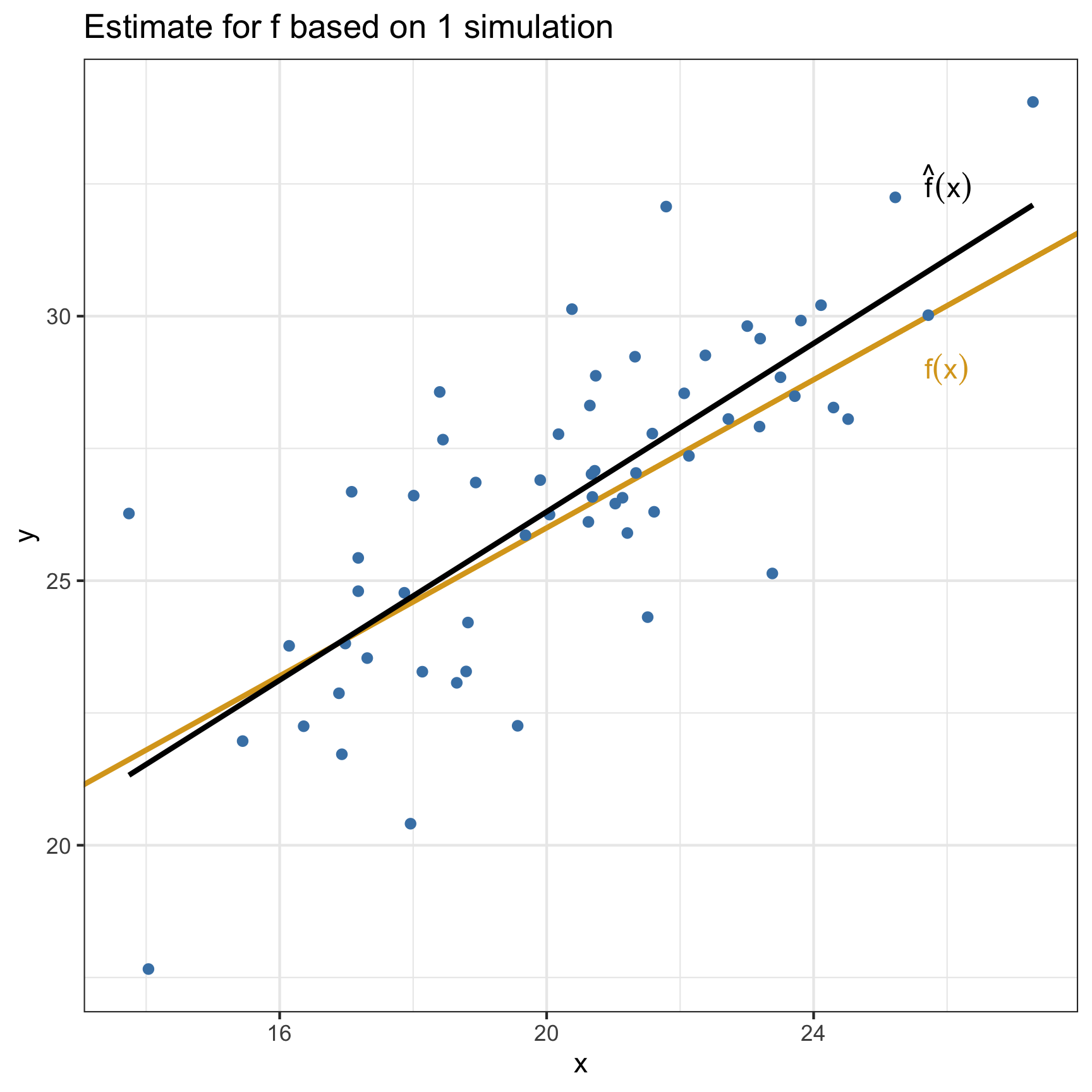
Assume the following true model: \[ f(x) = 12 + 0.7 x; \quad \epsilon \sim N(0, 4) \]

ggplot(my_data, 
       aes(x = x, y = y)) +
  geom_abline(slope = beta_1,
              intercept = 12,
              color = "goldenrod",
              size = 1) +
  geom_point(color = "steelblue")+
  geom_smooth(method = "lm",
              se = F,
              color = "black") +
  theme_bw() +
  annotate("text", x = 26, y = 29, label = "f(x)", color = "goldenrod", parse = T) +
  annotate("text", x = 26, y = 32.5, label = "hat(f)(x)", color = "black", parse = T) +
  labs(title = "Estimate for f based on 1 simulation")
The Sampling Distribution of \(\hat{\beta}_1\)

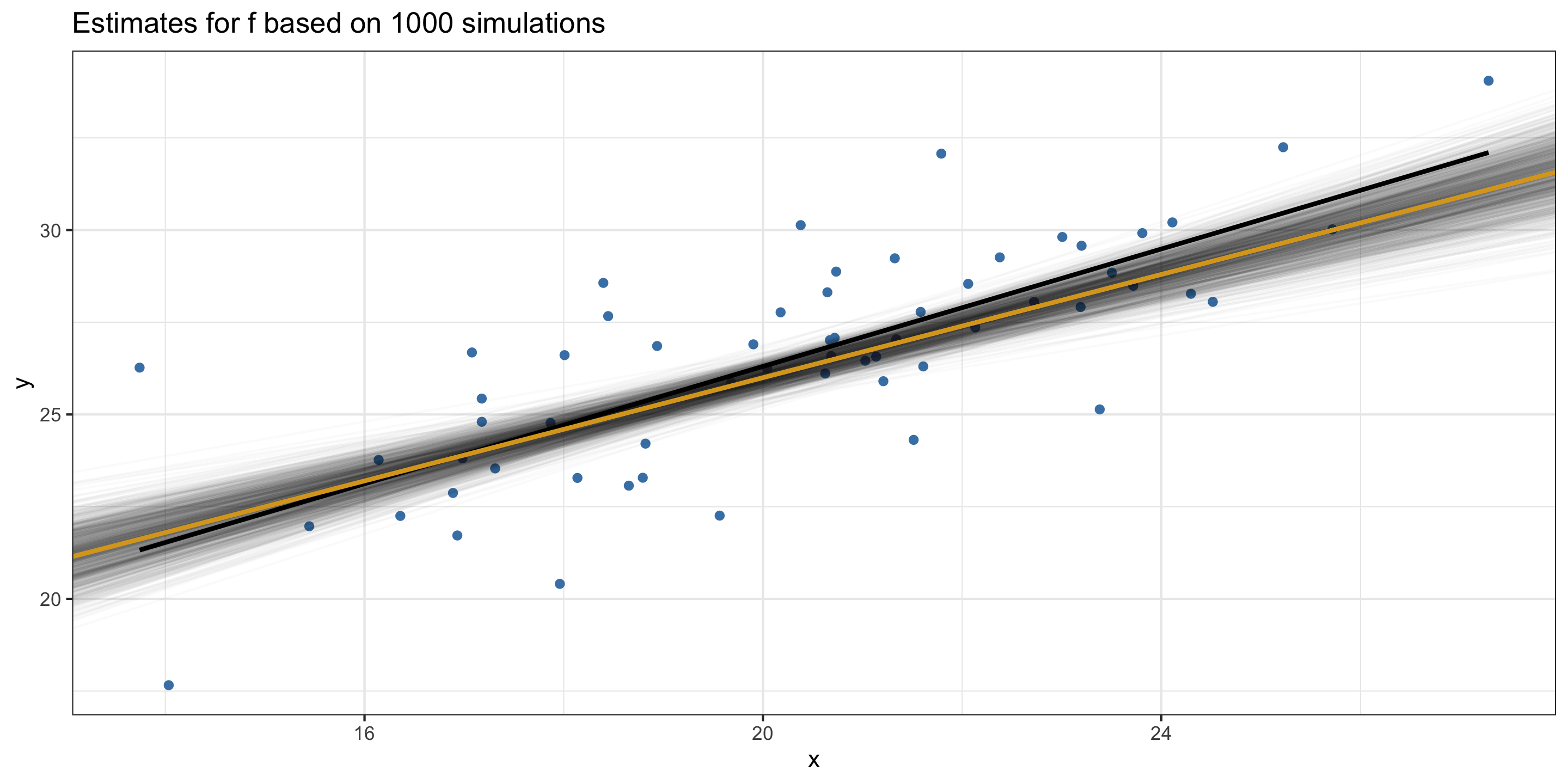
Assume the following true model: \[ f(x) = 12 + 0.7 x; \quad \epsilon \sim N(0, 4) \]

set.seed(1020)
it <- 1000
slope <- rep(NA, times = it)
intercept <- rep(NA, times = it)
for(i in 1:it) {
  x <- rnorm(n, mean = 20, sd = 3)
  f_mean <- beta_0 + beta_1 * x
  y <- f_mean + rnorm(n, mean = 0, sd = sigma)
  slope[i] <- lm(y ~ x)$coef[[2]]
  intercept[i] <- lm(y ~ x)$coef[[1]]
}
many_mods <- data.frame(slope, intercept)

ggplot(my_data, 
       aes(x = x, y = y)) +
  geom_point(color = "steelblue") +
  geom_abline(data = many_mods, 
              slope = slope, 
              intercept = intercept, 
              alpha = .02) +
  geom_smooth(method = "lm",
              se = F,
              color = "black") +
  geom_abline(slope = beta_1,
              intercept = 12,
              color = "goldenrod",
              size = 1) +
  theme_bw() +
  labs(title = "Estimates for f based on 1000 simulations")
The Sampling Distribution of \(\hat{\beta}_1\)
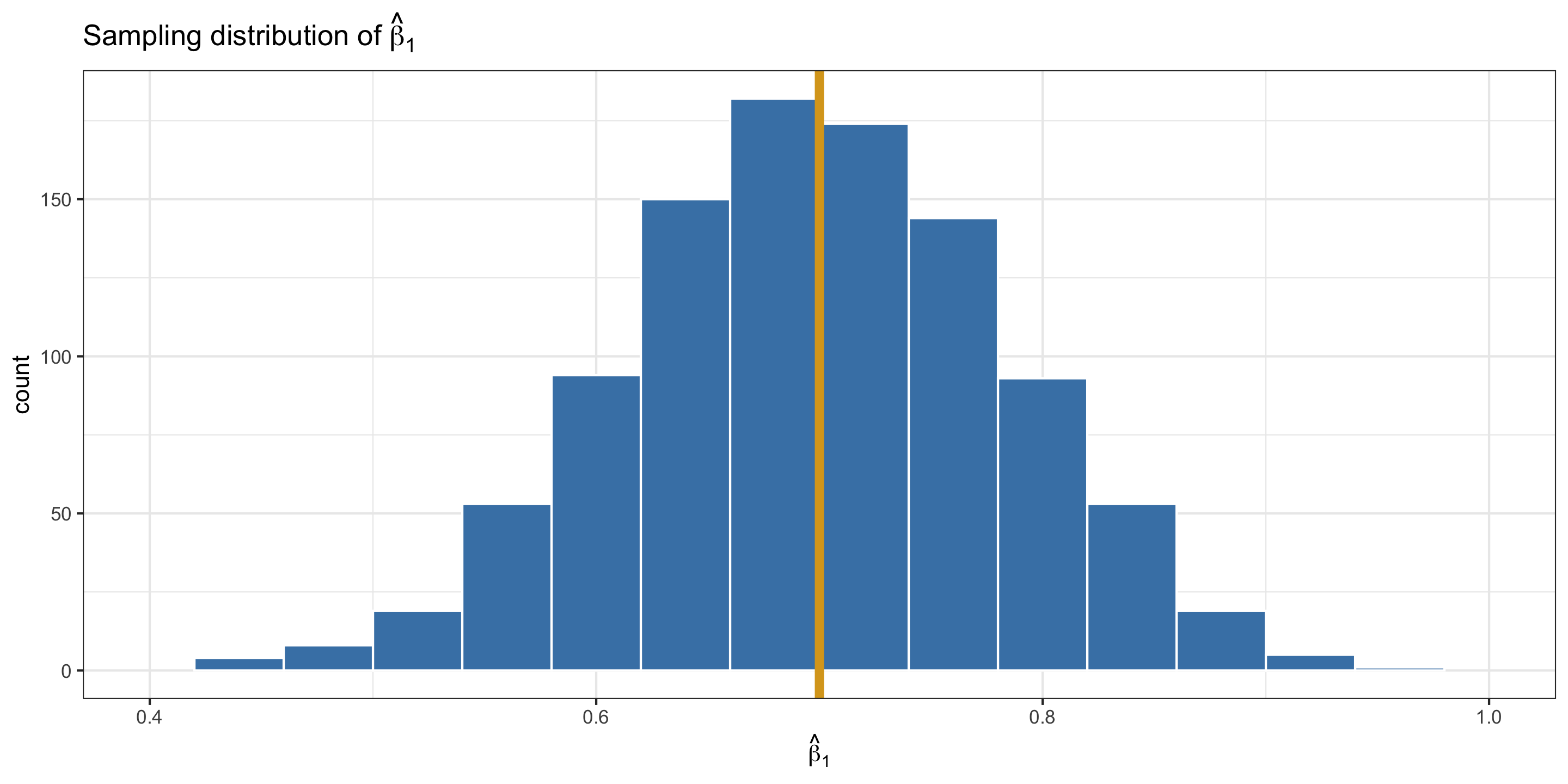
The Sampling Distribution of \(\hat{\beta}_1\)
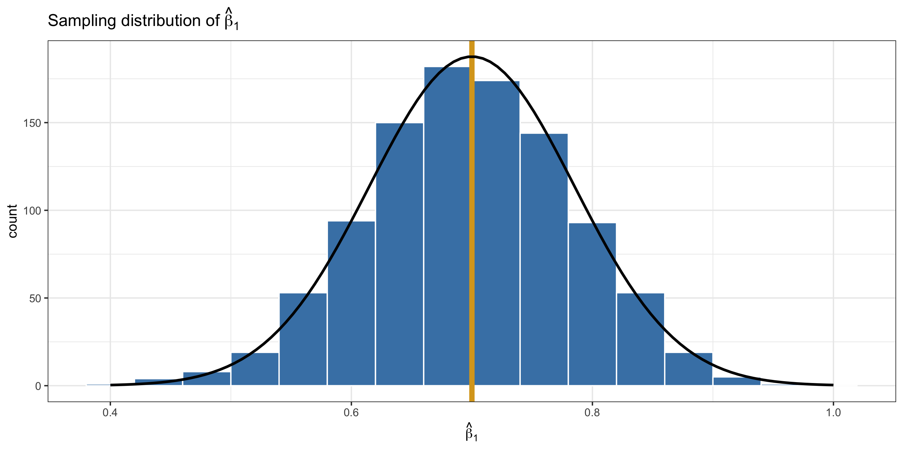
The Sampling Distribution of \(\hat{\beta}_1\)

The Sampling Distribution of \(\hat{\beta}_1\)

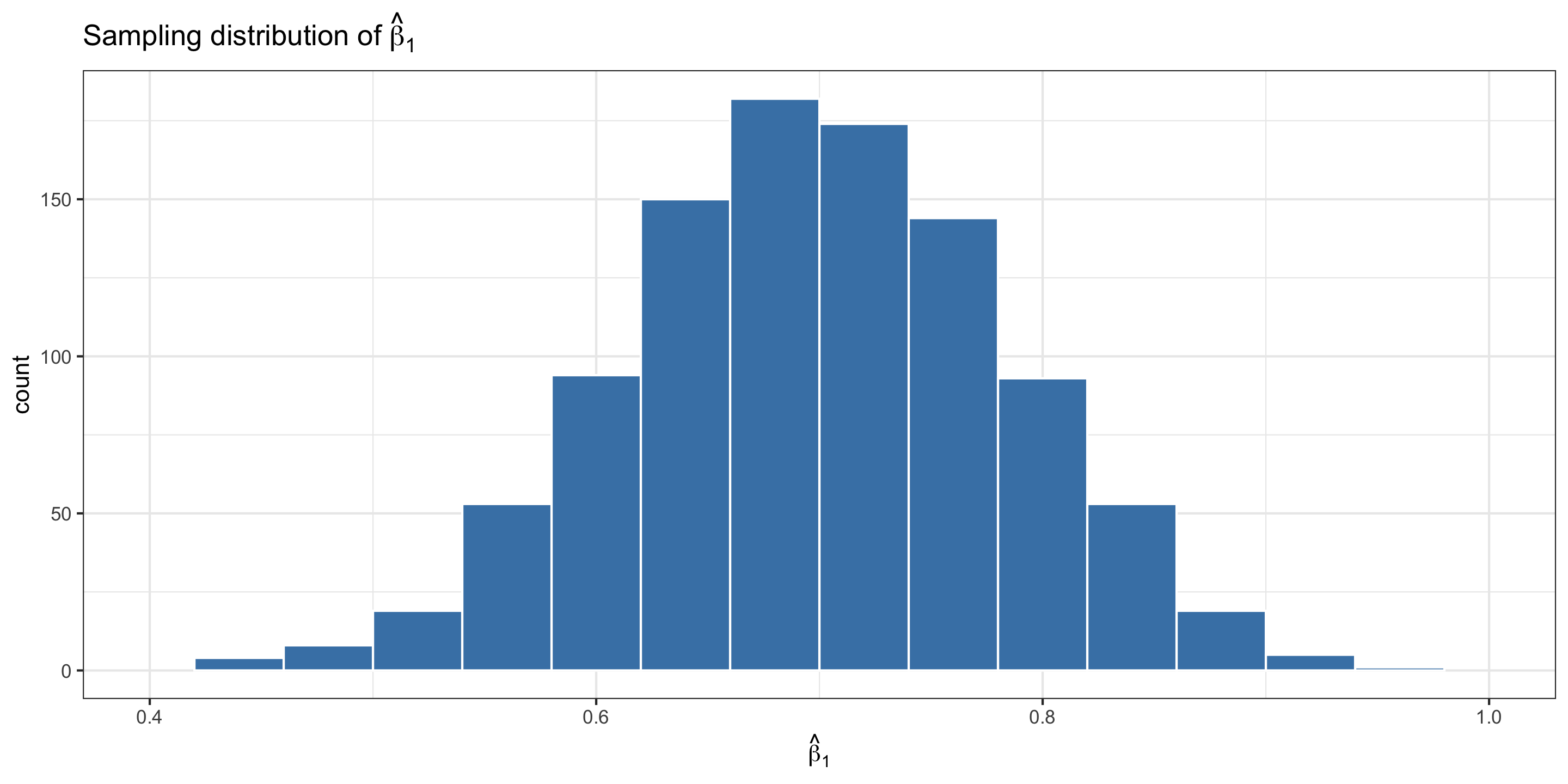
The Sampling Distribution has the following characteristics:

  1. Centered at \(\beta_1\), i.e. \(\mathbb{E}(\hat{\beta}_1) = \beta_1\).

  2. \(\mbox{Var}(\hat{\beta}_1) = \frac{\sigma^2}{S_{XX}}\).

    • where \(S_{XX} = \sum_{i = 1}^n (x_i - \bar{x})^2\)
  3. \(\hat{\beta}_1 | X \sim N (\beta_1, \frac{\sigma^2}{S_{XX}})\).

Who cares?

  • We need facts about the sampling distribution to do two main tasks:
    • build confidence intervals, and
    • perform hypothesis tests.

Building a confidence interval

We’d like to use the sampling distribution to build a CI for \(\beta\):

\[ \hat{\beta} \pm t^*_C \cdot \widehat{\mathrm{SE}}(\hat{\beta}) \]

  • Our best estimate of \(\beta_1\) is \(\hat{\beta}_1\) (since the expected value \(\hat \beta_1\) is \(\beta_1\))

  • However, we need to estimate \(\mbox{SE}(\hat\beta)\). How to do this?

  • Use the sampling distribution!! (Why can’t we?)

  • In reality we never have access to the true sampling distribution. Instead we approximate it by:

    • Assuming it follows a distributional form, or
    • Using simulation (e.g., the bootstrap)

Building a confidence interval for \(\hat{\beta}_1\)

  • In reality we never have access to the true sampling distribution. Instead we approximate it by:
    • Assuming it follows a distributional form, or
    • Using simulation (bootstrap)

Distributional assumptions

\[\widehat{\mbox{SE}}(\hat{\beta}_1) = \frac{\hat \sigma}{\sqrt{\sum_{i=1}^n(x_i - \bar x)^2}}\]

  • For linear regression, reasonable if we (1) meet the LINE conditions, and (2) have a sample size >30.

Simulation (bootstrap)

Use the percentile or standard error method to estimate \(\mbox{SE}(\hat\beta_1)\) from estimates of \(\beta_1\) from many bootstrap samples.

  • For linear regression, reasonable if we (1) meet Linearity and Independence, and (2) have a sample size >30.

Performing a hypothesis test for \(\hat{\beta}_1\)

Suppose we are interested in testing the claim that the slope is zero.

\[ H_0: \beta_1 = 0 \qquad \textrm{vs} \quad H_A: \beta_1 \ne 0 \]

  • Two options: use simulation (permutation), or make distributional assumptions.

Distributional assumptions

Consider the statistic \(t\) given by \[ t = \frac{\hat{\beta}_1}{\widehat{\mbox{SE}}(\hat{\beta}_1)} \]

  • \(t \sim t(\mbox{df} = n-2)\) and \(SE(\hat{\beta}_1)\) calculated the same as in the CI.

  • For linear regression, reasonable if we (1) meet the LINE conditions, and (2) have a sample size >30.

Simulation (permutation)

Use the percentile or standard error method to estimate \(\mbox{SE}(\hat\beta_1)\) from estimates of \(\beta_1\) from many permutations of your original dataset.

  • For linear regression, reasonable if we meet Linearity and Independence. No sample size restriction

Categorical Predictors

What About A Categorical Explanatory Variable?

  • Response variable \((y)\): quantitative

  • Have 1 categorical explanatory variable \((x)\) with two categories.

  • Model form:

\[ \begin{align} y &= \beta_o + \beta_1 x + \epsilon \end{align} \]

  • First, need to convert the categories of \(x\) to numbers.

Example: Halloween Candy

candy <- read_csv("https://raw.githubusercontent.com/fivethirtyeight/data/master/candy-power-ranking/candy-data.csv")
glimpse(candy)
Rows: 85
Columns: 13
$ competitorname   <chr> "100 Grand", "3 Musketeers", "One dime", "One quarter…
$ chocolate        <dbl> 1, 1, 0, 0, 0, 1, 1, 0, 0, 0, 1, 0, 0, 0, 0, 0, 0, 0,…
$ fruity           <dbl> 0, 0, 0, 0, 1, 0, 0, 0, 0, 1, 0, 1, 1, 1, 1, 1, 1, 1,…
$ caramel          <dbl> 1, 0, 0, 0, 0, 0, 1, 0, 0, 1, 0, 0, 0, 0, 0, 0, 0, 0,…
$ peanutyalmondy   <dbl> 0, 0, 0, 0, 0, 1, 1, 1, 0, 0, 0, 0, 0, 0, 0, 0, 0, 0,…
$ nougat           <dbl> 0, 1, 0, 0, 0, 0, 1, 0, 0, 0, 1, 0, 0, 0, 0, 0, 0, 0,…
$ crispedricewafer <dbl> 1, 0, 0, 0, 0, 0, 0, 0, 0, 0, 0, 0, 0, 0, 0, 0, 0, 0,…
$ hard             <dbl> 0, 0, 0, 0, 0, 0, 0, 0, 0, 0, 0, 0, 0, 0, 1, 0, 1, 1,…
$ bar              <dbl> 1, 1, 0, 0, 0, 1, 1, 0, 0, 0, 1, 0, 0, 0, 0, 0, 0, 0,…
$ pluribus         <dbl> 0, 0, 0, 0, 0, 0, 0, 1, 1, 0, 0, 1, 1, 1, 0, 1, 0, 1,…
$ sugarpercent     <dbl> 0.732, 0.604, 0.011, 0.011, 0.906, 0.465, 0.604, 0.31…
$ pricepercent     <dbl> 0.860, 0.511, 0.116, 0.511, 0.511, 0.767, 0.767, 0.51…
$ winpercent       <dbl> 66.97173, 67.60294, 32.26109, 46.11650, 52.34146, 50.…

What might be a good categorical explanatory variable of winpercent?

Exploratory Data Analysis

Before building the model, let’s explore and visualize the data!

  • What dplyr functions should I use to find the mean and sd of winpercent by the categories of chocolate?

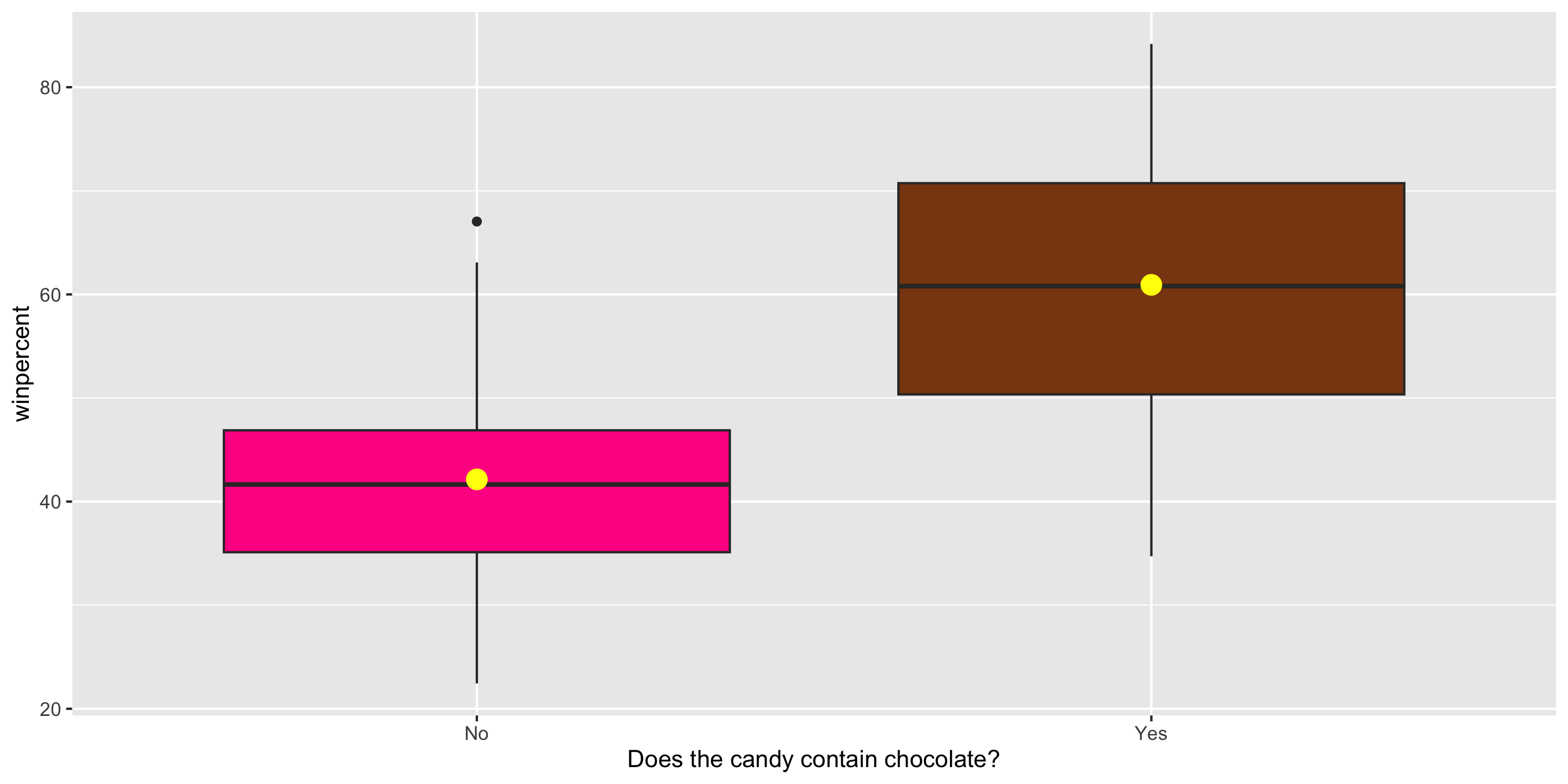
  • What graph should we use to visualize the winpercent scores by chocolate?

Exploratory Data Analysis

# Summarize
candy %>%
  group_by(chocolate) %>%
  summarize(count = n(),
            mean_win = mean(winpercent), 
            sd_win = sd(winpercent))
# A tibble: 2 × 4
  chocolate count mean_win sd_win
      <dbl> <int>    <dbl>  <dbl>
1         0    48     42.1   10.2
2         1    37     60.9   12.8

Exploratory Data Analysis

ggplot(candy, aes(x = factor(chocolate), 
                   y = winpercent, 
                  fill = factor(chocolate))) +
  geom_boxplot() +
  stat_summary(fun = mean,
               geom = "point",
               color = "yellow",
               size = 4) +
  guides(fill = "none") +
  scale_fill_manual(values =
                      c("0" = "deeppink",
                        "1" = "chocolate4")) +
  scale_x_discrete(labels = c("No", "Yes"),
                   name =
          "Does the candy contain chocolate?")
Fit the Linear Regression Model

Model Form:

\[ \begin{align} y &= \beta_o + \beta_1 x + \epsilon \end{align} \]

When \(x = 0\): \(\qquad y = \beta_o + \epsilon\)


When \(x = 1\): \(\qquad y = \beta_o + \beta_1 + \epsilon\)

mod <- lm(winpercent ~ chocolate, data = candy)
library(moderndive)
get_regression_table(mod)
# A tibble: 2 × 7
  term      estimate std_error statistic p_value lower_ci upper_ci
  <chr>        <dbl>     <dbl>     <dbl>   <dbl>    <dbl>    <dbl>
1 intercept     42.1      1.65     25.6        0     38.9     45.4
2 chocolate     18.8      2.50      7.52       0     13.8     23.7

Notes

  • When the explanatory variable is categorical, \(\beta_o\) and \(\beta_1\) no longer represent the intercept and slope.

  • Now \(\beta_o\) represents the (population) mean of the response variable when \(x = 0\).

  • And, \(\beta_1\) represents the change in the (population) mean response going from \(x = 0\) to \(x = 1\).

  • Can also do prediction:

new_candy <- data.frame(chocolate = c(0, 1))
predict(mod, newdata = new_candy)
       1        2 
42.14226 60.92153 

New example: Palmer Penguins

library(palmerpenguins)

Take a look at the data

glimpse(penguins)
Rows: 344
Columns: 8
$ species           <fct> Adelie, Adelie, Adelie, Adelie, Adelie, Adelie, Adel…
$ island            <fct> Torgersen, Torgersen, Torgersen, Torgersen, Torgerse…
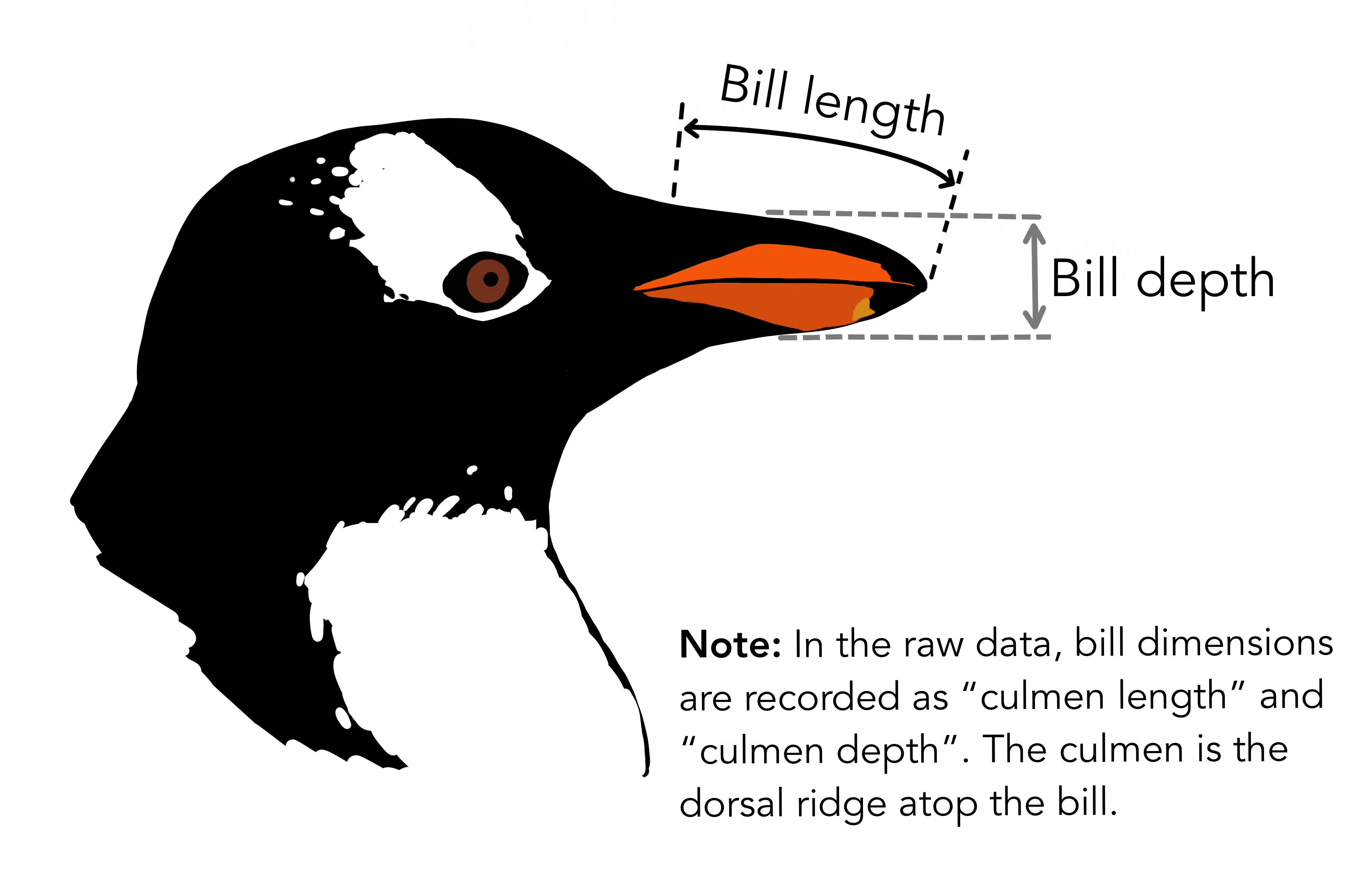
$ bill_length_mm    <dbl> 39.1, 39.5, 40.3, NA, 36.7, 39.3, 38.9, 39.2, 34.1, …
$ bill_depth_mm     <dbl> 18.7, 17.4, 18.0, NA, 19.3, 20.6, 17.8, 19.6, 18.1, …
$ flipper_length_mm <int> 181, 186, 195, NA, 193, 190, 181, 195, 193, 190, 186…
$ body_mass_g       <int> 3750, 3800, 3250, NA, 3450, 3650, 3625, 4675, 3475, …
$ sex               <fct> male, female, female, NA, female, male, female, male…
$ year              <int> 2007, 2007, 2007, 2007, 2007, 2007, 2007, 2007, 2007…

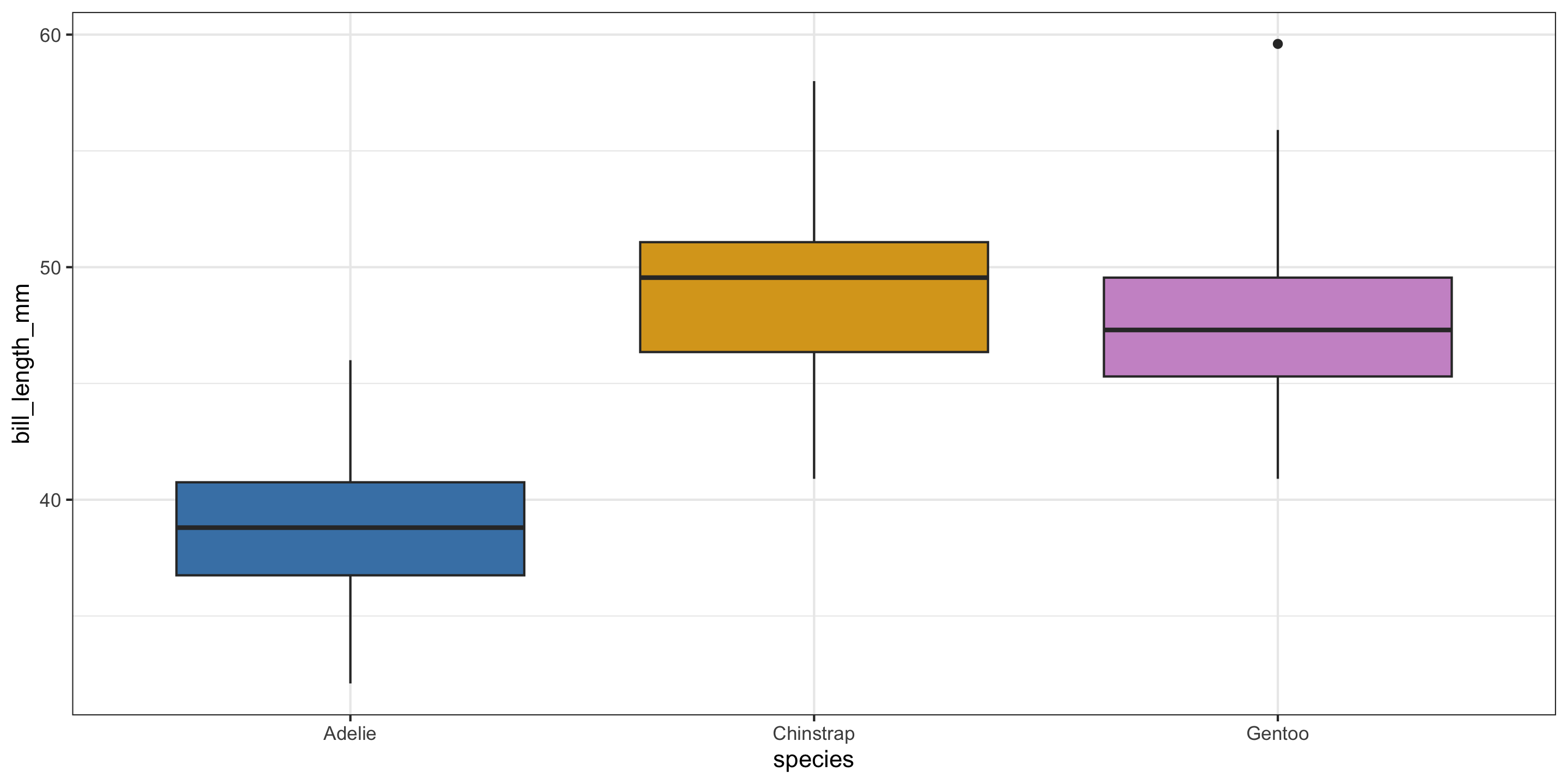
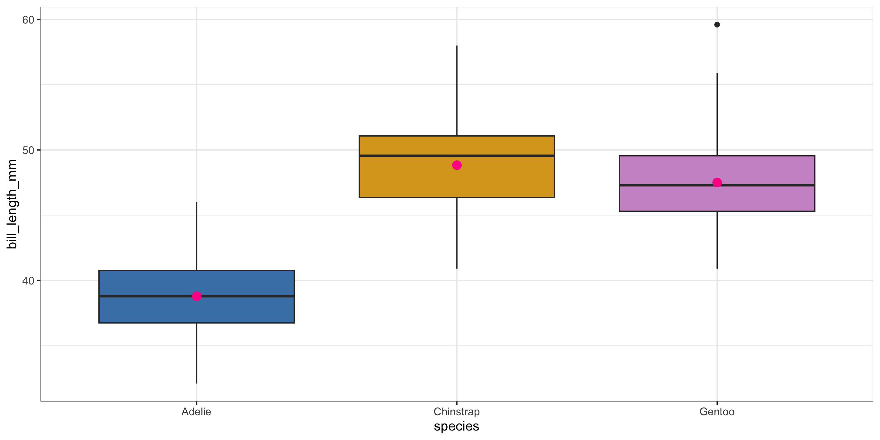
We’d like to predict a penguin’s bill length based on their species.
Response variable?

Explanatory variable?

Exploratory data analysis

penguins %>%
  group_by(species) %>%
  summarize(
    avg_bill_length = mean(bill_length_mm,
                           na.rm = TRUE)
    )
# A tibble: 3 × 2
  species   avg_bill_length
  <fct>               <dbl>
1 Adelie               38.8
2 Chinstrap            48.8
3 Gentoo               47.5
ggplot(penguins, 
       aes(x = species,
           y = bill_length_mm, 
           fill = species)) +
  geom_boxplot() +
  scale_fill_manual(values = c("steelblue",
                               "goldenrod", 
                               "plum3")) +
  guides(fill = "none") +
  theme_bw()

How do we handle more than 2 groups???

Boardwork

Fit the model in R

\[ y = \beta_o + \beta_1 x_{species:Chinstrap} + \beta_2 x_{species:Gentoo} + \epsilon \]

penguin_mod <- lm(bill_length_mm ~ species, penguins)
get_regression_table(penguin_mod)
# A tibble: 3 × 7
  term               estimate std_error statistic p_value lower_ci upper_ci
  <chr>                 <dbl>     <dbl>     <dbl>   <dbl>    <dbl>    <dbl>
1 intercept             38.8      0.241     161.        0    38.3     39.3 
2 species: Chinstrap    10.0      0.432      23.2       0     9.19    10.9 
3 species: Gentoo        8.71     0.36       24.2       0     8.01     9.42

\[\begin{align*} \hat{y} &= \hat{\beta}_o + \hat{\beta}_1 \cdot x_{species:Chinstrap} + \hat{\beta}_2 \cdot x_{species:Gentoo} \\ &= 38.8 + 10.0 \cdot x_{species:Chinstrap} + 8.71 \cdot x_{species:Gentoo} \end{align*}\]

Coefficient interpretation?

Multiple Linear Regression

Before:

We predicted a penguin’s bill length based on their species.

ggplot(penguins, aes(x = species, y = bill_length_mm, fill = species)) +
  geom_boxplot() + 
  scale_fill_manual(values = c("steelblue",
                               "goldenrod", 
                               "plum3")) +
  stat_summary(fun = mean, 
               geom = "point", 
               size = 3,
               color = "deeppink") + 
  guides(fill = "none") +
  theme_bw()

  • Pink dots represent the mean value in each group.
  • For the single categorical variable model, those pink dots are the predicted values for each group.

Now:

We’ll incorporate bill depth for prediction!
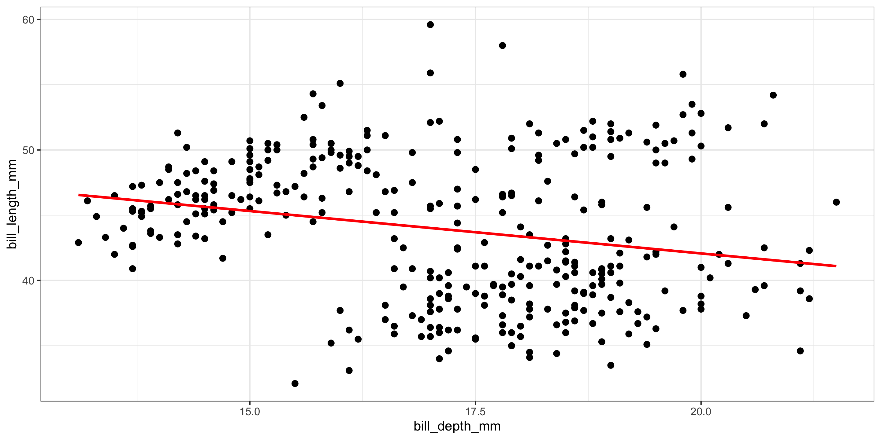
ggplot(penguins, aes(x = bill_depth_mm, y = bill_length_mm)) +
  geom_point(size = 2) + 
  geom_smooth(method = "lm", se = FALSE, color = "red") + 
  theme_bw()

  • A moderate negative relationship between bill length and bill depth!
  • Does this make sense?

What if we include both explanatory variables?

ggplot(penguins, aes(x = bill_depth_mm, y = bill_length_mm, color = species)) +
  geom_point(size = 2) + 
  geom_smooth(inherit.aes = FALSE, 
              mapping = aes(x = bill_depth_mm,
                            y = bill_length_mm),
              method = "lm",
              se = FALSE,
              color = "red") + 
  geom_parallel_slopes(se = FALSE) + 
  scale_color_manual(values = c("steelblue",
                               "goldenrod", 
                               "plum3")) +
  theme_bw() +
  theme(legend.position = "bottom")
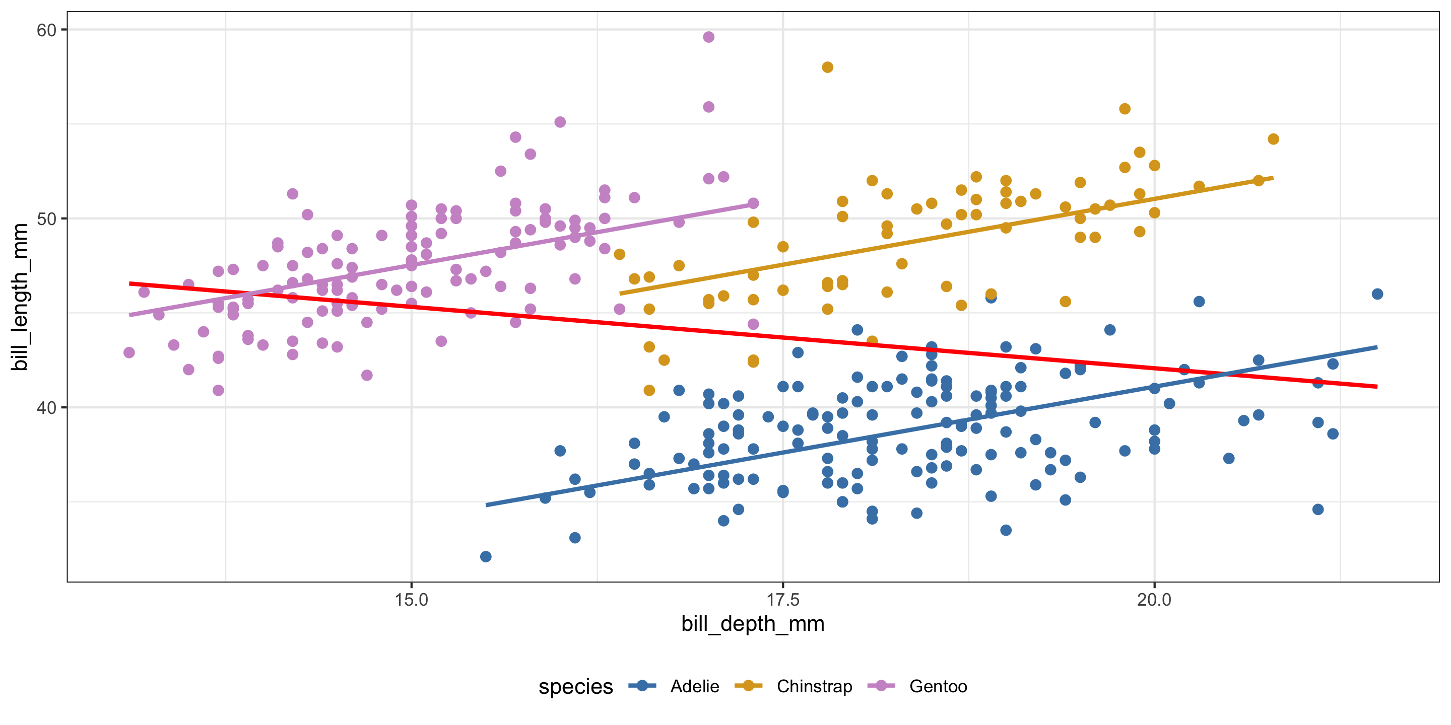
  • Negative relationships between bill depth and bill length overall.
  • Positive relationships between bill depth and bill length when accounting for species!
  • What is going on here??
  • This is a case of Simpson’s Paradox.

Three candidate models

species_mod <- lm(bill_length_mm ~ species, penguins)
get_regression_table(species_mod) %>%
  select(term, estimate)
# A tibble: 3 × 2
  term               estimate
  <chr>                 <dbl>
1 intercept             38.8 
2 species: Chinstrap    10.0 
3 species: Gentoo        8.71


depth_mod <- lm(bill_length_mm ~ bill_depth_mm, penguins)
get_regression_table(depth_mod) %>%
  select(term, estimate)
# A tibble: 2 × 2
  term          estimate
  <chr>            <dbl>
1 intercept        55.1 
2 bill_depth_mm    -0.65


both_mod <- lm(bill_length_mm ~ bill_depth_mm + species, penguins)
get_regression_table(both_mod) %>%
  select(term, estimate)
# A tibble: 4 × 2
  term               estimate
  <chr>                 <dbl>
1 intercept             13.2 
2 bill_depth_mm          1.39
3 species: Chinstrap     9.94
4 species: Gentoo       13.4 
  • Coefficient interpretations?

Interpreting the Multiple Regression Equation

get_regression_table(both_mod)
# A tibble: 4 × 7
  term               estimate std_error statistic p_value lower_ci upper_ci
  <chr>                 <dbl>     <dbl>     <dbl>   <dbl>    <dbl>    <dbl>
1 intercept             13.2      2.25       5.88       0     8.80    17.6 
2 bill_depth_mm          1.39     0.122     11.4        0     1.15     1.63
3 species: Chinstrap     9.94     0.368     27.0        0     9.22    10.7 
4 species: Gentoo       13.4      0.512     26.2        0    12.4     14.4 

\[ \hat{y}= 13.2 + 1.39 \cdot x_{\textrm{Bill Depth}} + 9.94 \cdot x_{\textrm{Species:Chinstrap}} + 13.4 \cdot x_{\textrm{Species:Gentoo}} \]

  • Slope Coefficient on Quantitative Variable: The expected/predicted change in response variable, on average, per unit increase in the explanatory variable, holding all other variables constant.
    • Example: We expect a 1.394mm increase in bill length for every 1mm increase in bill depth, on average, after holding species constant.

Interpreting the Multiple Regression Equation

get_regression_table(both_mod)
# A tibble: 4 × 7
  term               estimate std_error statistic p_value lower_ci upper_ci
  <chr>                 <dbl>     <dbl>     <dbl>   <dbl>    <dbl>    <dbl>
1 intercept             13.2      2.25       5.88       0     8.80    17.6 
2 bill_depth_mm          1.39     0.122     11.4        0     1.15     1.63
3 species: Chinstrap     9.94     0.368     27.0        0     9.22    10.7 
4 species: Gentoo       13.4      0.512     26.2        0    12.4     14.4 

\[ \hat{y}= 13.2 + 1.39 \cdot x_{\textrm{Bill Depth}} + 9.94 \cdot x_{\textrm{Species:Chinstrap}} + 13.4 \cdot x_{\textrm{Species:Gentoo}} \]

  • Intercept Coefficient: The expected/predicted value of the response, on average, when all explanatory variables are set to 0.
    • What does setting species to 0 mean in this context?

Returning to our MLR model

ggplot(penguins, aes(x = bill_depth_mm, y = bill_length_mm, color = species)) +
  geom_point(size = 2) + 
  geom_parallel_slopes(se = FALSE) + 
  scale_color_manual(values = c("steelblue",
                               "goldenrod", 
                               "plum3")) +
  theme_bw() 

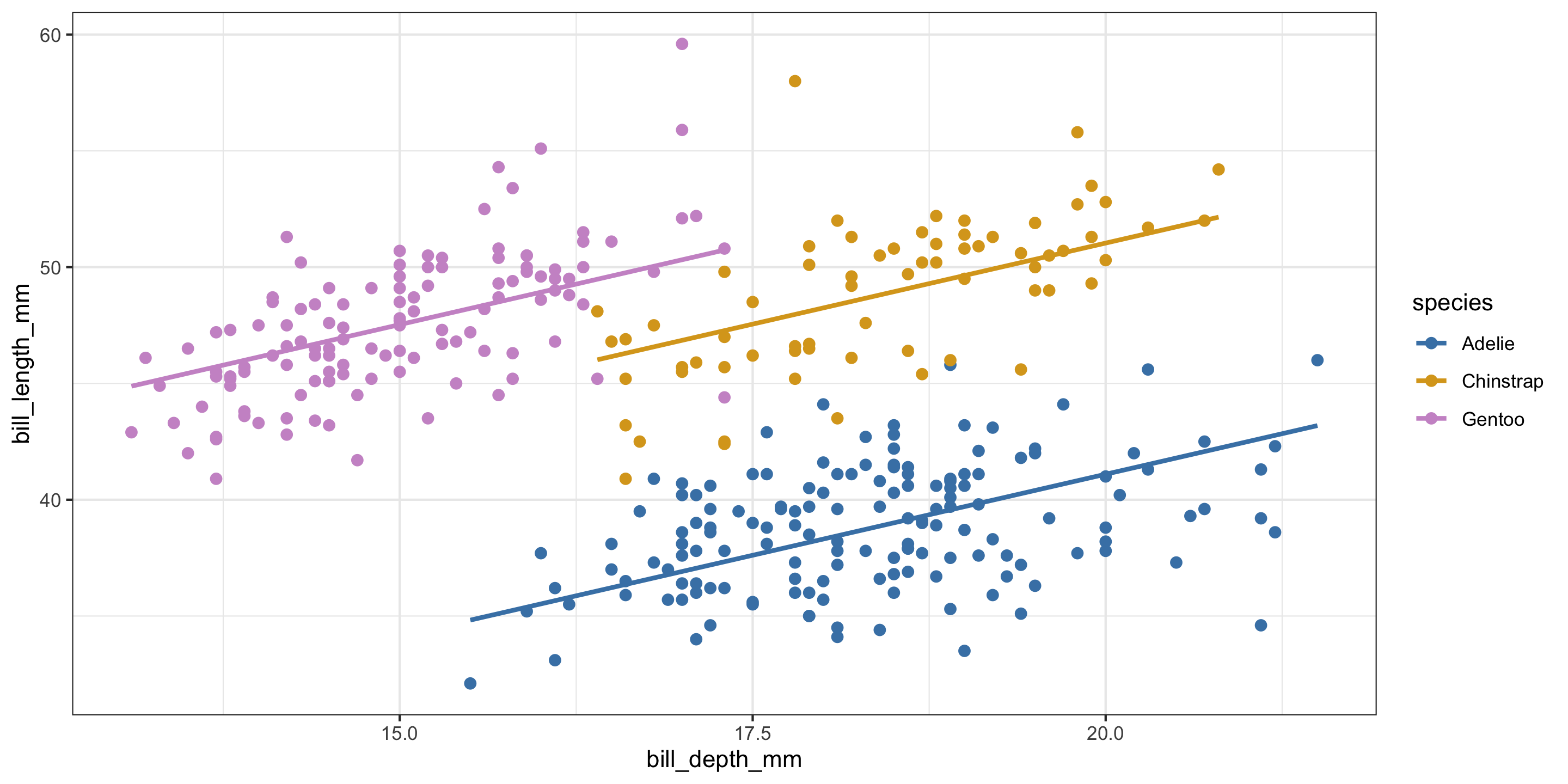
Are equal slopes a reasonable assumption here?

Different Slopes Model
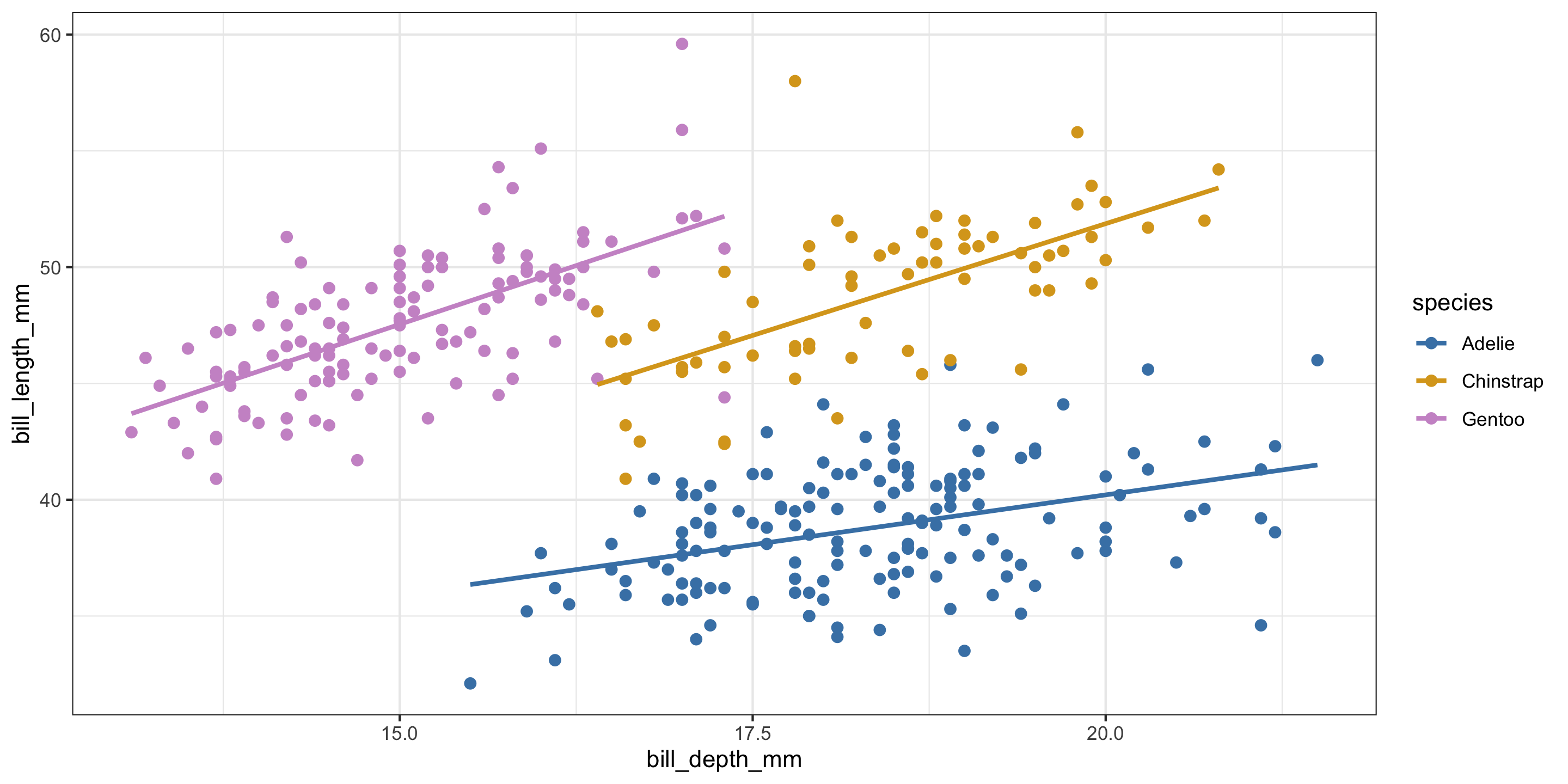
ggplot(penguins, aes(x = bill_depth_mm, y = bill_length_mm, color = species)) +
  geom_point(size = 2) + 
  geom_smooth(method = "lm", se = FALSE) + 
  scale_color_manual(values = c("steelblue",
                               "goldenrod", 
                               "plum3")) +
  theme_bw() 

  • Equal slopes models force the relationship between quantitative predictors and the response variable to be the same for each group in the model.

  • In contrast, different slopes models allow for different relationships between quantitative predictors and the response variable for each group in the model.

  • How can we allow our model to have different slopes?

Contrasting model forms

Recall the equal slopes model:

\[ y = \beta_o + \beta_1 \cdot x_{\textrm{Bill Depth}} + \beta_2 \cdot x_{\textrm{Species:Chinstrap}} + \beta_3 \cdot x_{\textrm{Species:Gentoo}} + \epsilon \]


How can we allow the slopes to vary?

\[ y = \beta_o + \beta_1 \cdot x_{\textrm{Bill Depth}} + \beta_2 \cdot x_{\textrm{Species:Chinstrap}} + \beta_3 \cdot x_{\textrm{Species:Gentoo}} + \\ \beta_4 \cdot x_{\textrm{Bill Depth}} \cdot x_{\textrm{Species:Chinstrap}} + \beta_5 \cdot x_{\textrm{Bill Depth}} \cdot x_{\textrm{Species:Gentoo}} + \epsilon \]

  • Coefficient interpretation?

Different Slopes Model in R

same_slope <- lm(bill_length_mm ~ bill_depth_mm + species, penguins)

diff_slope <- lm(bill_length_mm ~ bill_depth_mm * species, penguins)
get_regression_table(same_slope)
# A tibble: 4 × 7
  term               estimate std_error statistic p_value lower_ci upper_ci
  <chr>                 <dbl>     <dbl>     <dbl>   <dbl>    <dbl>    <dbl>
1 intercept             13.2      2.25       5.88       0     8.80    17.6 
2 bill_depth_mm          1.39     0.122     11.4        0     1.15     1.63
3 species: Chinstrap     9.94     0.368     27.0        0     9.22    10.7 
4 species: Gentoo       13.4      0.512     26.2        0    12.4     14.4 


get_regression_table(diff_slope)
# A tibble: 6 × 7
  term                    estimate std_error statistic p_value lower_ci upper_ci
  <chr>                      <dbl>     <dbl>     <dbl>   <dbl>    <dbl>    <dbl>
1 intercept                 23.1       3.02       7.65   0       17.1      29.0 
2 bill_depth_mm              0.857     0.164      5.22   0        0.534     1.18
3 species: Chinstrap        -9.64      5.72      -1.69   0.093  -20.9       1.60
4 species: Gentoo           -5.84      4.54      -1.29   0.199  -14.8       3.08
5 bill_depth_mm:speciesC…    1.06      0.31       3.44   0.001    0.455     1.68
6 bill_depth_mm:speciesG…    1.16      0.279      4.17   0        0.615     1.71

How to assess which model is best?

  • Train-test split, check which minimizes MSE, bias, MAE, …