
Linear Regression II
Grayson White
Stat 243
Week 3 | Fall 2026
Today:
This Week:
\[ y = f(x) + \epsilon \]
Goal:
Determine a reasonable form for \(f()\). (Ex: Line, curve, …)
Estimate \(f()\) with \(\hat{f}()\) using the data.
Generate predicted values: \(\hat y = \hat{f}(x)\).
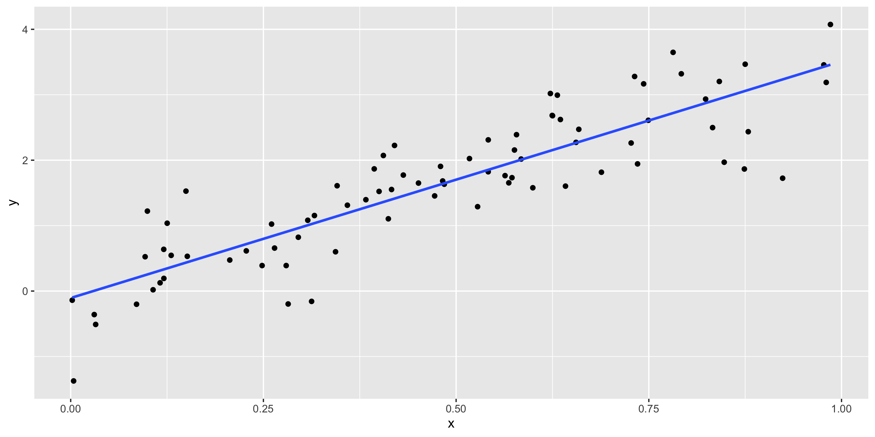
\[ y = \beta_o + \beta_1 x + \epsilon \]
Consider this model when:
Response variable \((y)\): quantitative
Explanatory variable \((x)\): quantitative
AND, \(f()\) can be approximated by a line.
Need to determine the best estimates of \(\beta_o\) and \(\beta_1\).
\[ y = \beta_o + \beta_1 x + \epsilon \]
\[ \hat{y} = \hat{ \beta}_o + \hat{\beta}_1 x \]
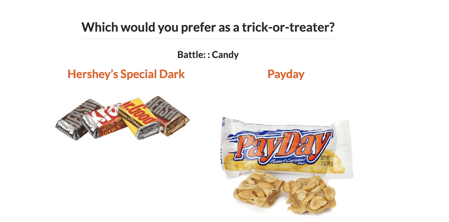
“The social contract of Halloween is simple: Provide adequate treats to costumed masses, or be prepared for late-night tricks from those dissatisfied with your offer. To help you avoid that type of vengeance, and to help you make good decisions at the supermarket this weekend, we wanted to figure out what Halloween candy people most prefer. So we devised an experiment: Pit dozens of fun-sized candy varietals against one another, and let the wisdom of the crowd decide which one was best.” – Walt Hickey
“While we don’t know who exactly voted, we do know this: 8,371 different IP addresses voted on about 269,000 randomly generated matchups. So, not a scientific survey or anything, but a good sample of what candy people like.”

Rows: 85
Columns: 13
$ competitorname <chr> "100 Grand", "3 Musketeers", "One dime", "One quarter…
$ chocolate <dbl> 1, 1, 0, 0, 0, 1, 1, 0, 0, 0, 1, 0, 0, 0, 0, 0, 0, 0,…
$ fruity <dbl> 0, 0, 0, 0, 1, 0, 0, 0, 0, 1, 0, 1, 1, 1, 1, 1, 1, 1,…
$ caramel <dbl> 1, 0, 0, 0, 0, 0, 1, 0, 0, 1, 0, 0, 0, 0, 0, 0, 0, 0,…
$ peanutyalmondy <dbl> 0, 0, 0, 0, 0, 1, 1, 1, 0, 0, 0, 0, 0, 0, 0, 0, 0, 0,…
$ nougat <dbl> 0, 1, 0, 0, 0, 0, 1, 0, 0, 0, 1, 0, 0, 0, 0, 0, 0, 0,…
$ crispedricewafer <dbl> 1, 0, 0, 0, 0, 0, 0, 0, 0, 0, 0, 0, 0, 0, 0, 0, 0, 0,…
$ hard <dbl> 0, 0, 0, 0, 0, 0, 0, 0, 0, 0, 0, 0, 0, 0, 1, 0, 1, 1,…
$ bar <dbl> 1, 1, 0, 0, 0, 1, 1, 0, 0, 0, 1, 0, 0, 0, 0, 0, 0, 0,…
$ pluribus <dbl> 0, 0, 0, 0, 0, 0, 0, 1, 1, 0, 0, 1, 1, 1, 0, 1, 0, 1,…
$ sugarpercent <dbl> 0.732, 0.604, 0.011, 0.011, 0.906, 0.465, 0.604, 0.31…
$ pricepercent <dbl> 86.0, 51.1, 11.6, 51.1, 51.1, 76.7, 76.7, 51.1, 32.5,…
$ winpercent <dbl> 66.97173, 67.60294, 32.26109, 46.11650, 52.34146, 50.…
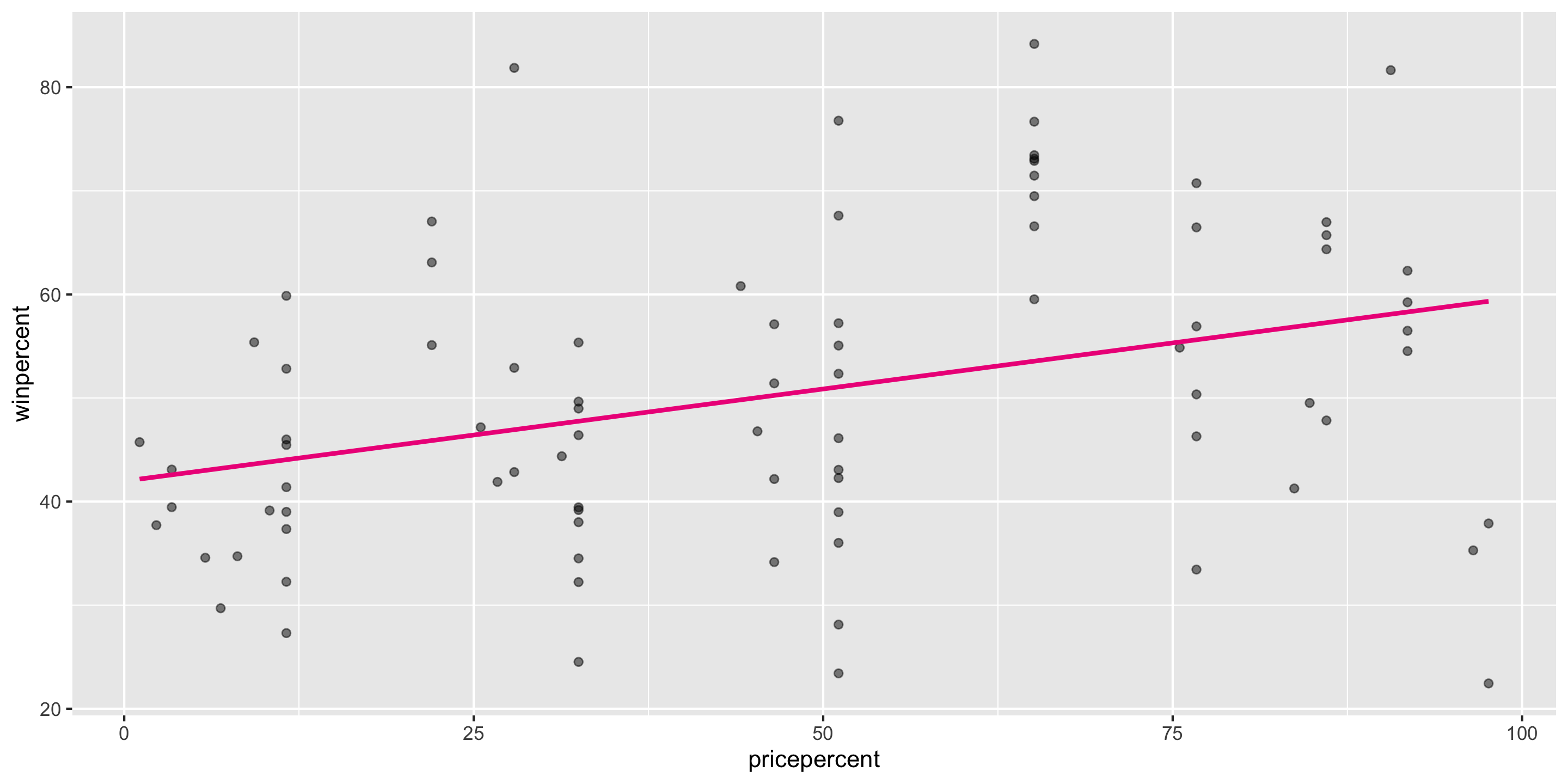
New modeling goal: predict win percentage by using the price percentage variable.
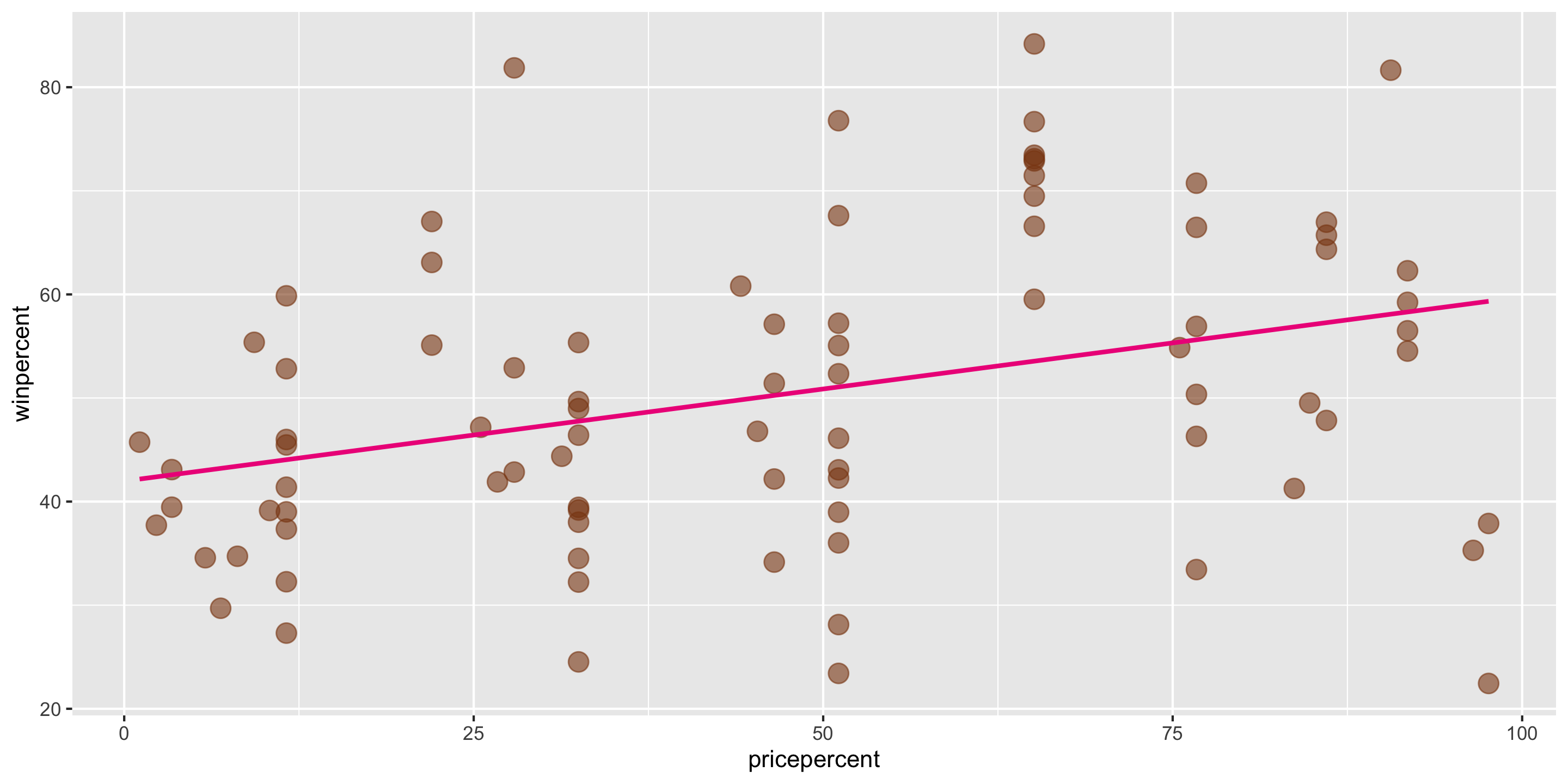
We can use the lm() function to construct the simple linear regression model in R.
# A tibble: 2 × 7
term estimate std_error statistic p_value lower_ci upper_ci
<chr> <dbl> <dbl> <dbl> <dbl> <dbl> <dbl>
1 intercept 41.979 2.908 14.435 0 36.195 47.763
2 pricepercent 0.178 0.053 3.352 0.001 0.072 0.283
What is the fitted model form?
\[\begin{align*} \hat{y} &= \hat{\beta_o} + \hat{\beta_1} \times x_{pricepercent} \\ &= 41.979 + 0.178 \times x_{pricepercent} \end{align*}\]
How do we interpret the coefficients?
1 2 3
46.42443 57.09409 68.65289
Careful to only predict values within the range of \(x\) values in the sample.
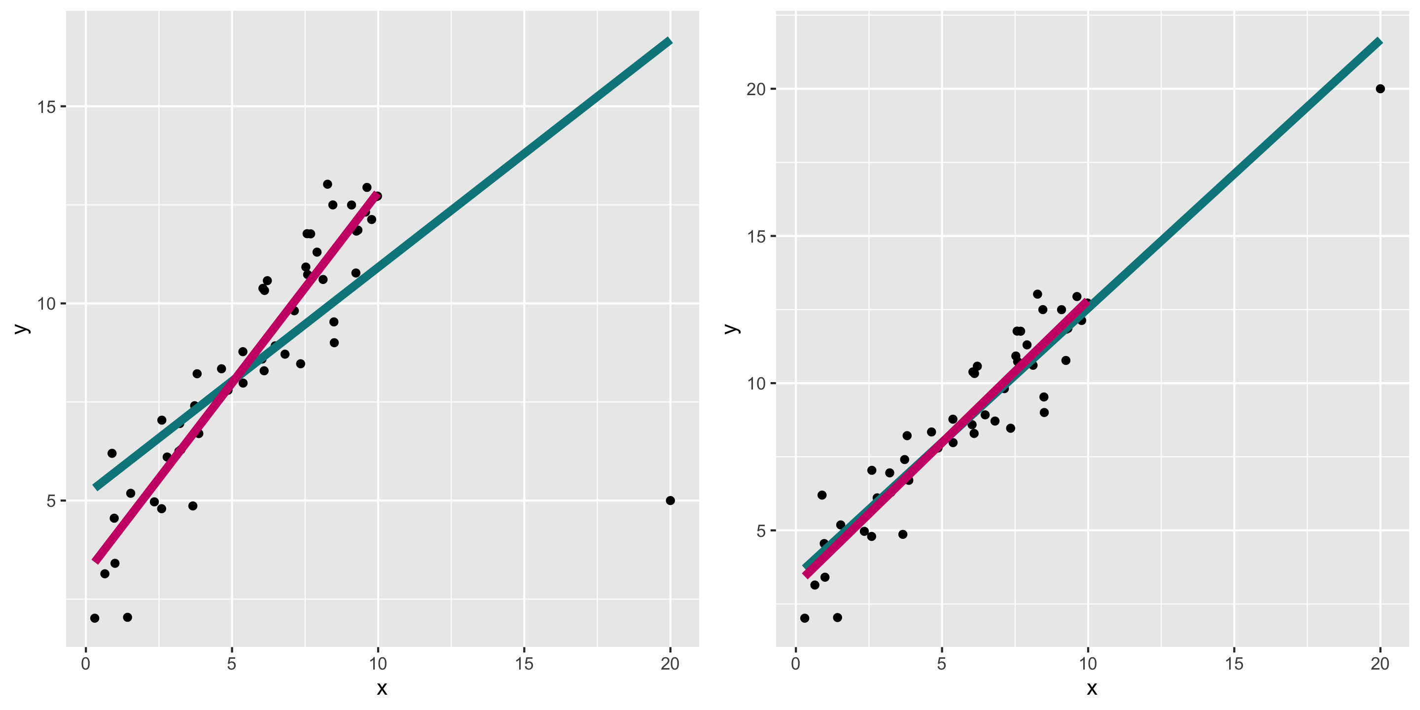
Make sure to investigate outliers: observations that fall far from the cloud of points.

# A tibble: 2 × 7
term estimate std_error statistic p_value lower_ci upper_ci
<chr> <dbl> <dbl> <dbl> <dbl> <dbl> <dbl>
1 intercept 41.979 2.908 14.435 0 36.195 47.763
2 pricepercent 0.178 0.053 3.352 0.001 0.072 0.283
\[\begin{align*} \hat{y} &= \hat{\beta_o} + \hat{\beta_1} \times x_{pricepercent} \\ &= 41.979 + 0.178 \times x_{pricepercent} \end{align*}\]
What assumptions have we made?
We can always find the line of best fit to explore data, but…
To make accurate predictions or inferences, certain conditions should be met.
\[\begin{align*} y &= \beta_o + \beta_1 + x + \epsilon \\ \epsilon &\overset{\mbox{ind}}{\sim} \mathcal{N}(0,~ \sigma^2) \end{align*}\]
Mathematically, all linear regression assumptions are encoded in the above equation.
However, we can break them down into four easy to remember mnemonics.
\[\begin{align*} y &= \beta_o + \beta_1 + x + \epsilon \\ \epsilon &\overset{\mbox{ind}}{\sim} \mathcal{N}(0,~ \sigma^2) \end{align*}\]
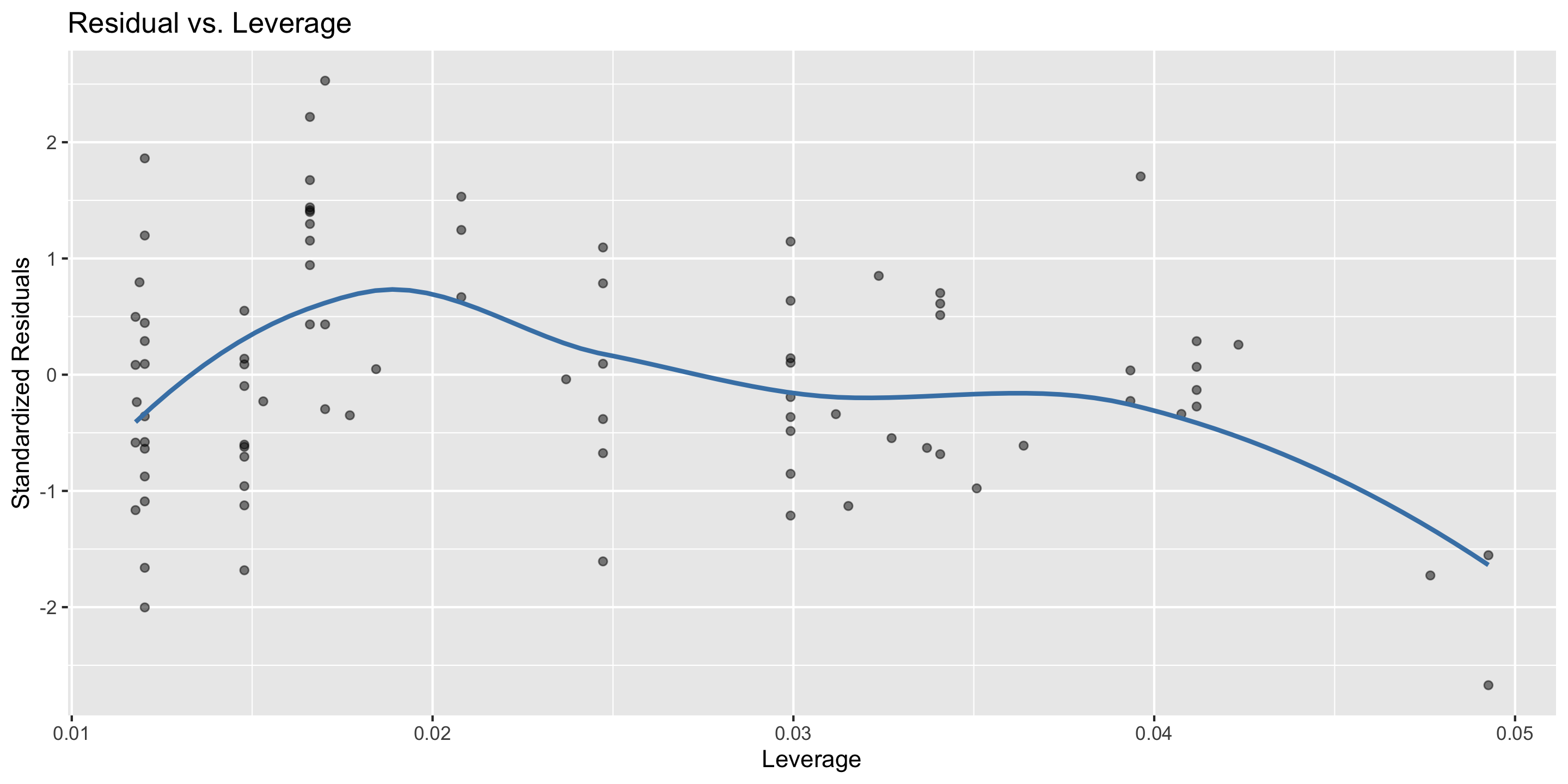
Linearity: The relationship between explanatory and response variables must be approximately linear
Mathematically: \(y = \beta_0 + \beta_1 x + \epsilon\) where \(\mathbb{E}(\epsilon \ | \ x) = 0\)
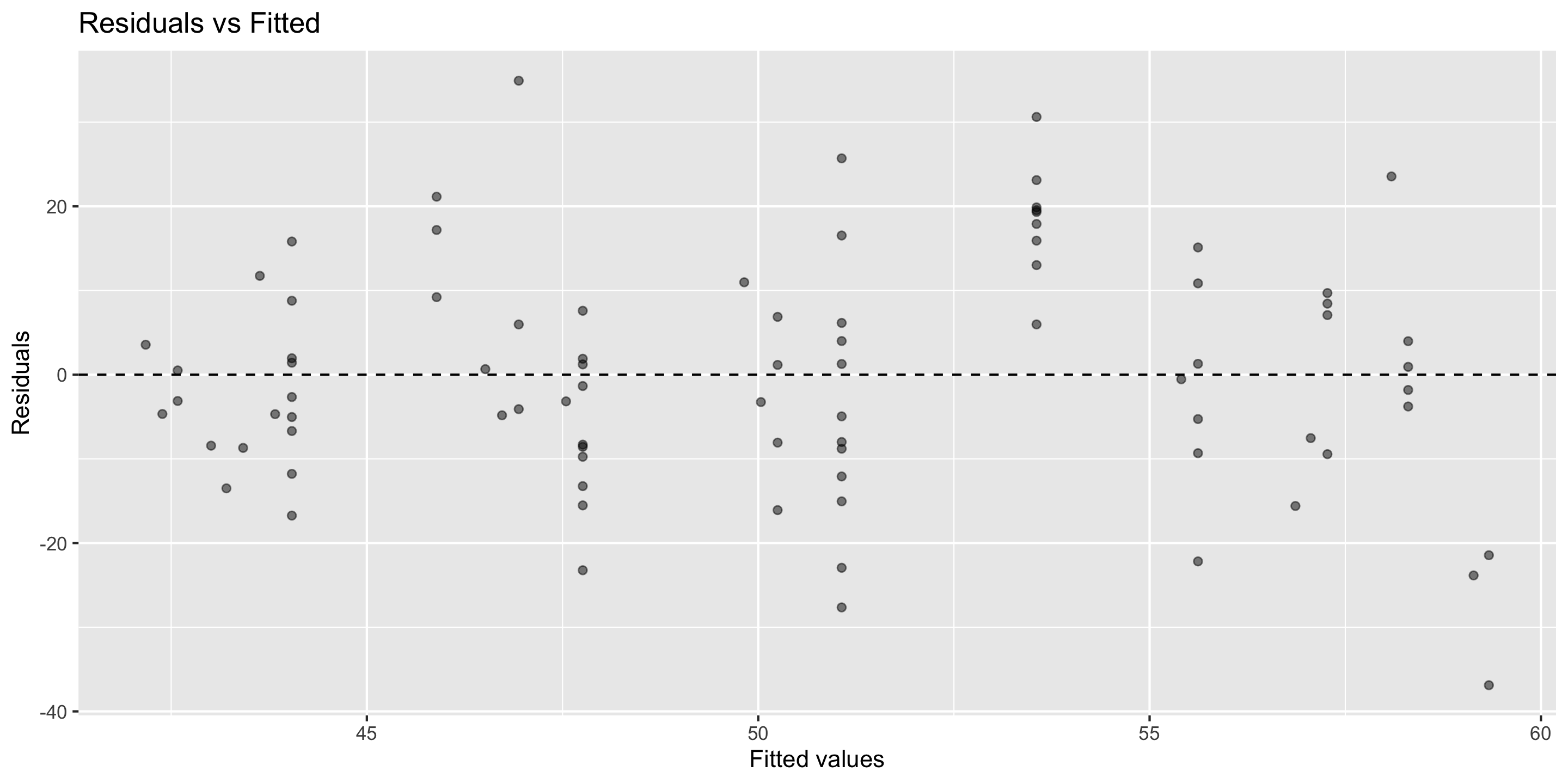
Check using scatterplot of data, or residual plot
\[\begin{align*} y &= \beta_o + \beta_1 + x + \epsilon \\ \epsilon &\overset{\mbox{ind}}{\sim} \mathcal{N}(0,~ \sigma^2) \end{align*}\]
Independence: The observations should be independent of one another.
\[\begin{align*} y &= \beta_o + \beta_1 + x + \epsilon \\ \epsilon &\overset{\mbox{ind}}{\sim} \mathcal{N}(0,~ \sigma^2) \end{align*}\]
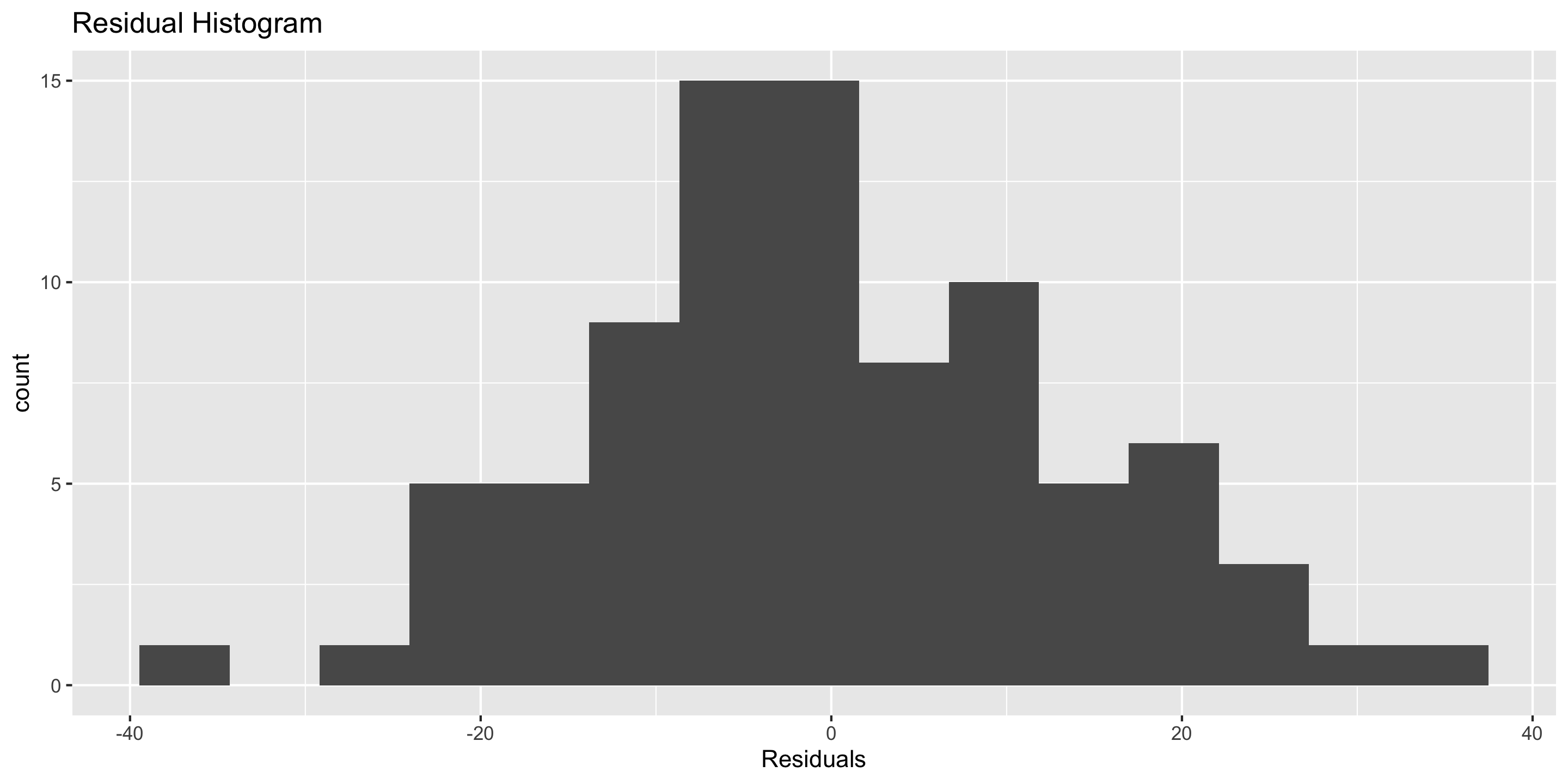
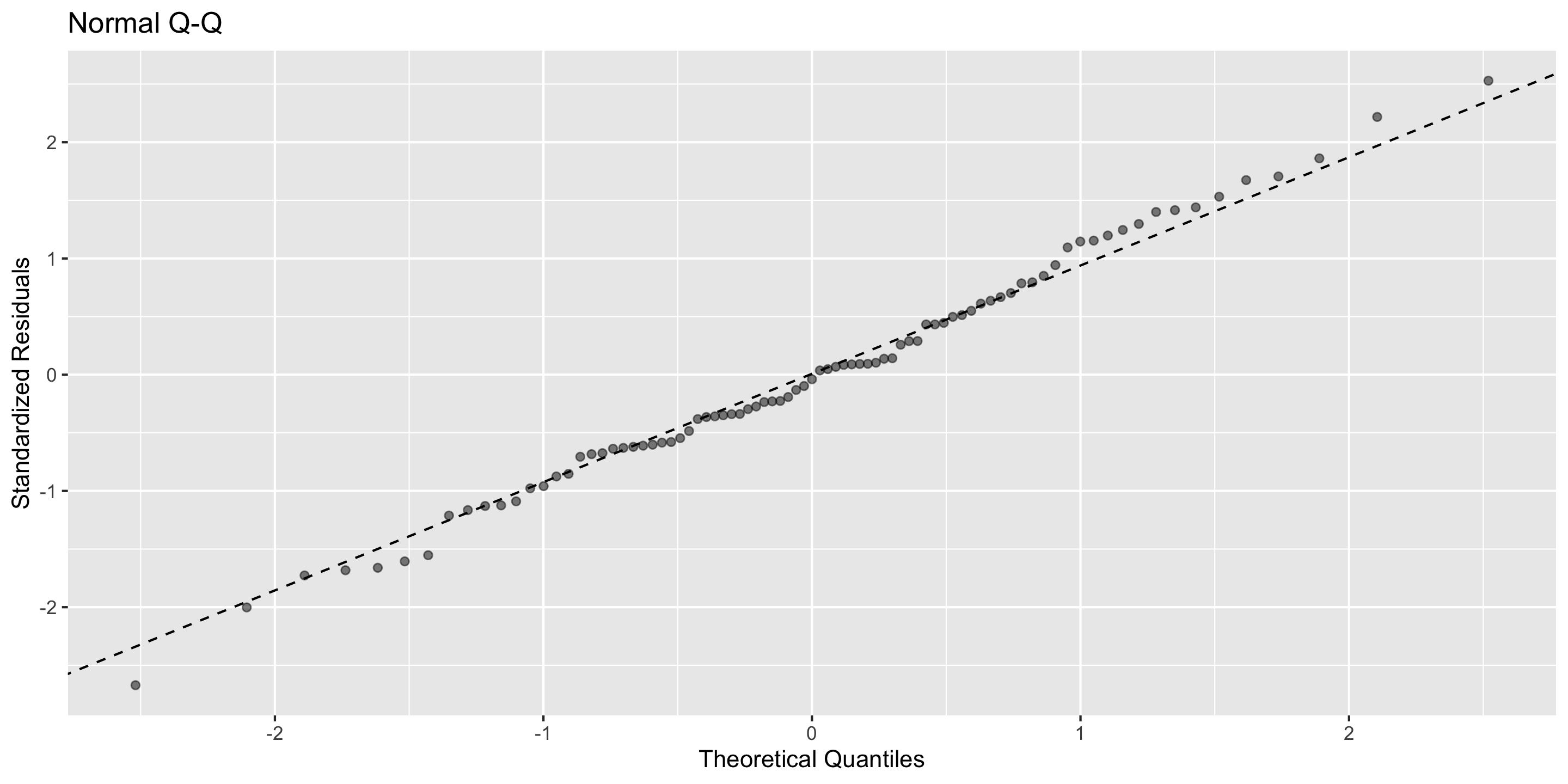
Normality: The distribution of residuals should be approximately bell-shaped, unimodal, symmetric, and centered at 0 at every “slice” of the explanatory variable
\[\begin{align*} y &= \beta_o + \beta_1 + x + \epsilon \\ \epsilon &\overset{\mbox{ind}}{\sim} \mathcal{N}(0,~ \sigma^2) \end{align*}\]
Equal Variability: Variance of residuals should be roughly constant across data set. Also called “homoscedasticity”. Models that violate this assumption are sometimes called “heteroscedastic”
Linearity: The relationship between explanatory and response variables must be approximately linear
Independence: The observations should be independent of one another.
Normality: The distribution of residuals should be approximately bell-shaped, unimodal, symmetric, and centered at 0 at every “slice” of the explanatory variable
Equal Variability: Variance of residuals should be roughly constant across data set. Also called “homoscedasticity”. Models that violate this assumption are sometimes called “heteroscedastic”
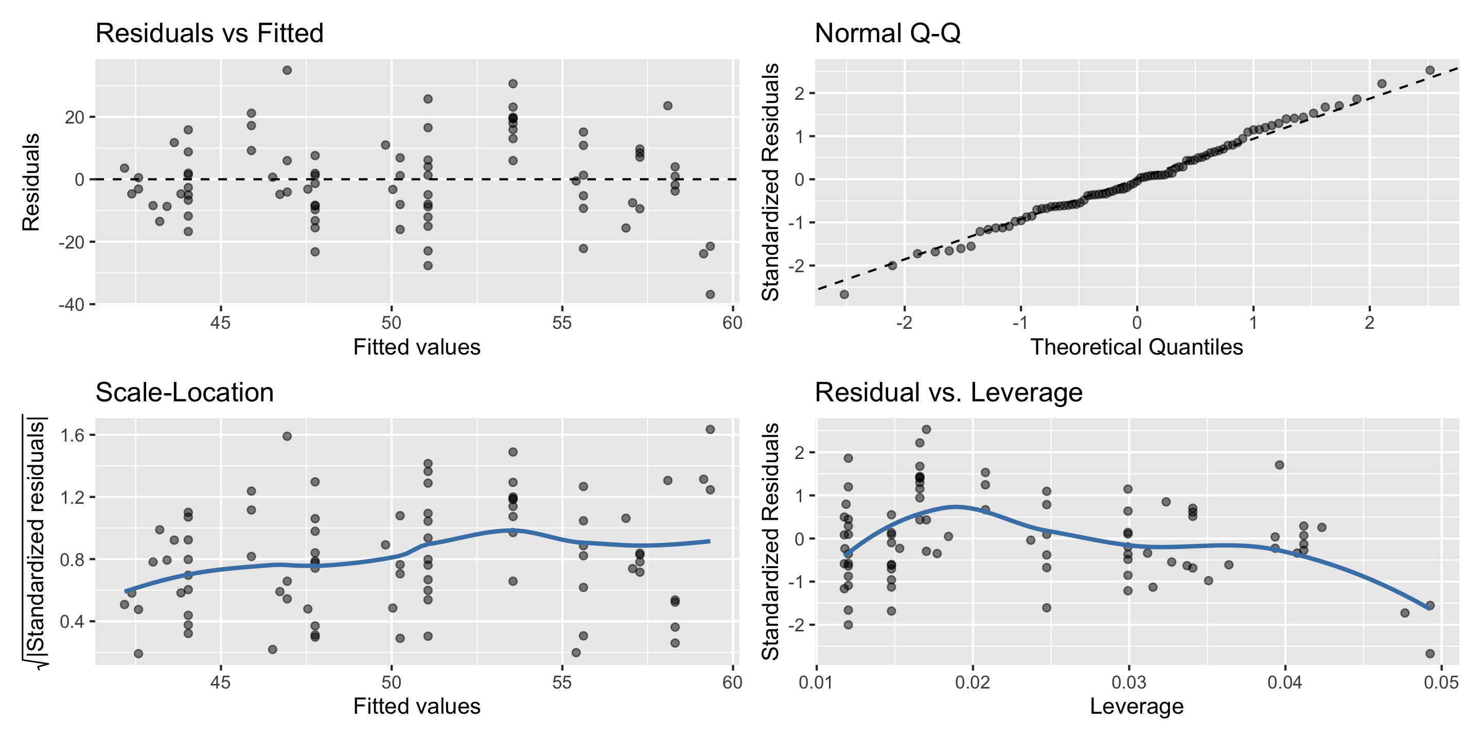
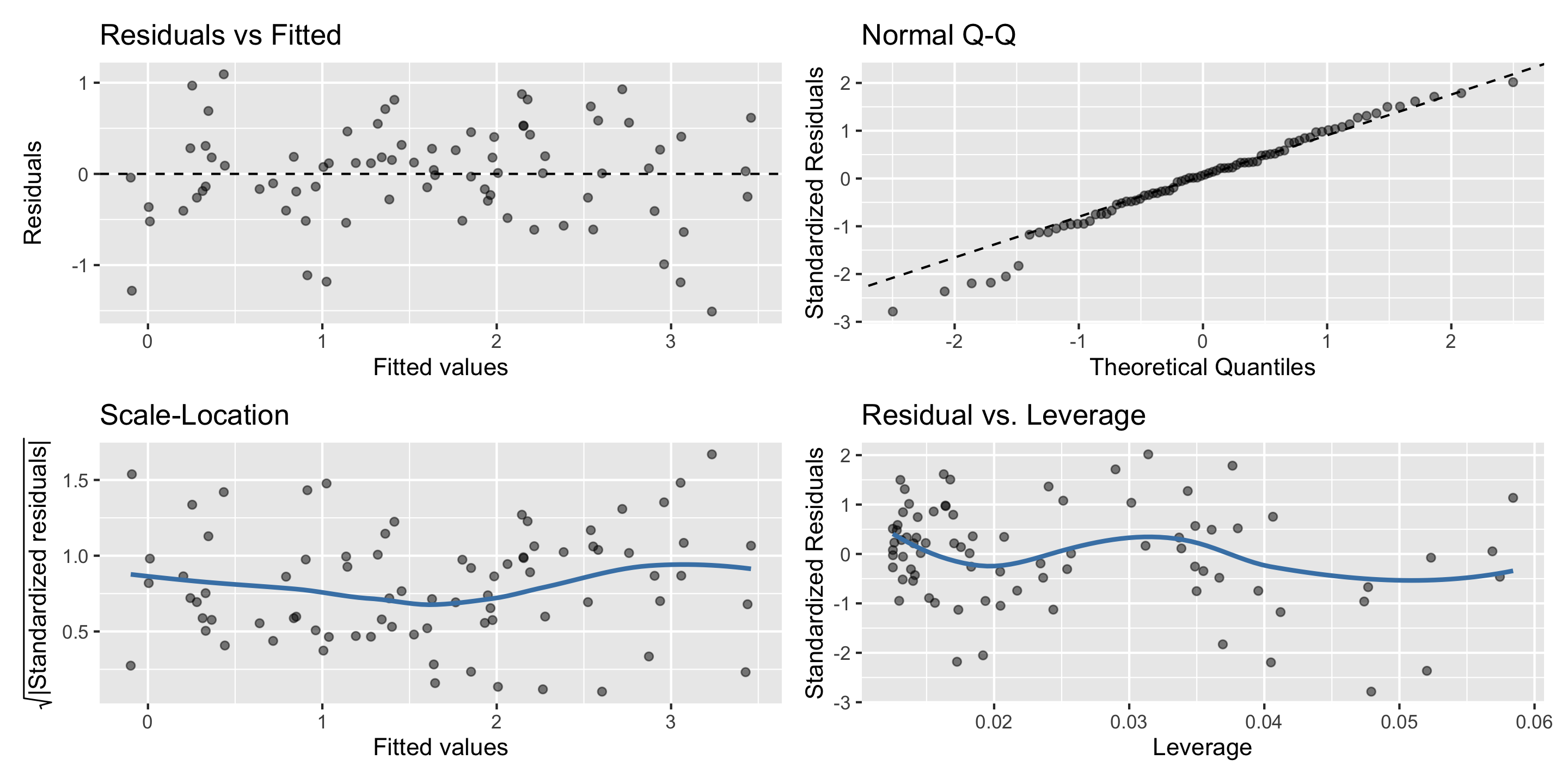
In order to assess if we’ve met the described conditions, we will utilize four common diagnostics plots:

Let’s check if this meets the LINE assumptions
Linearity: ✅
Independence: ✅
Equal Variability: ✅
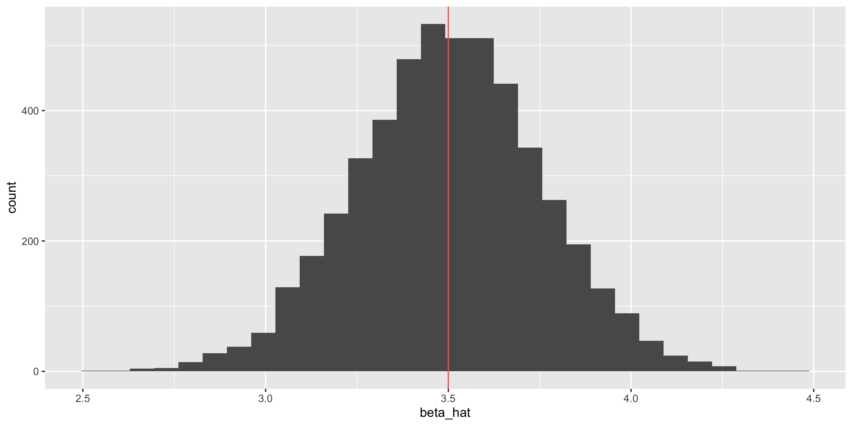
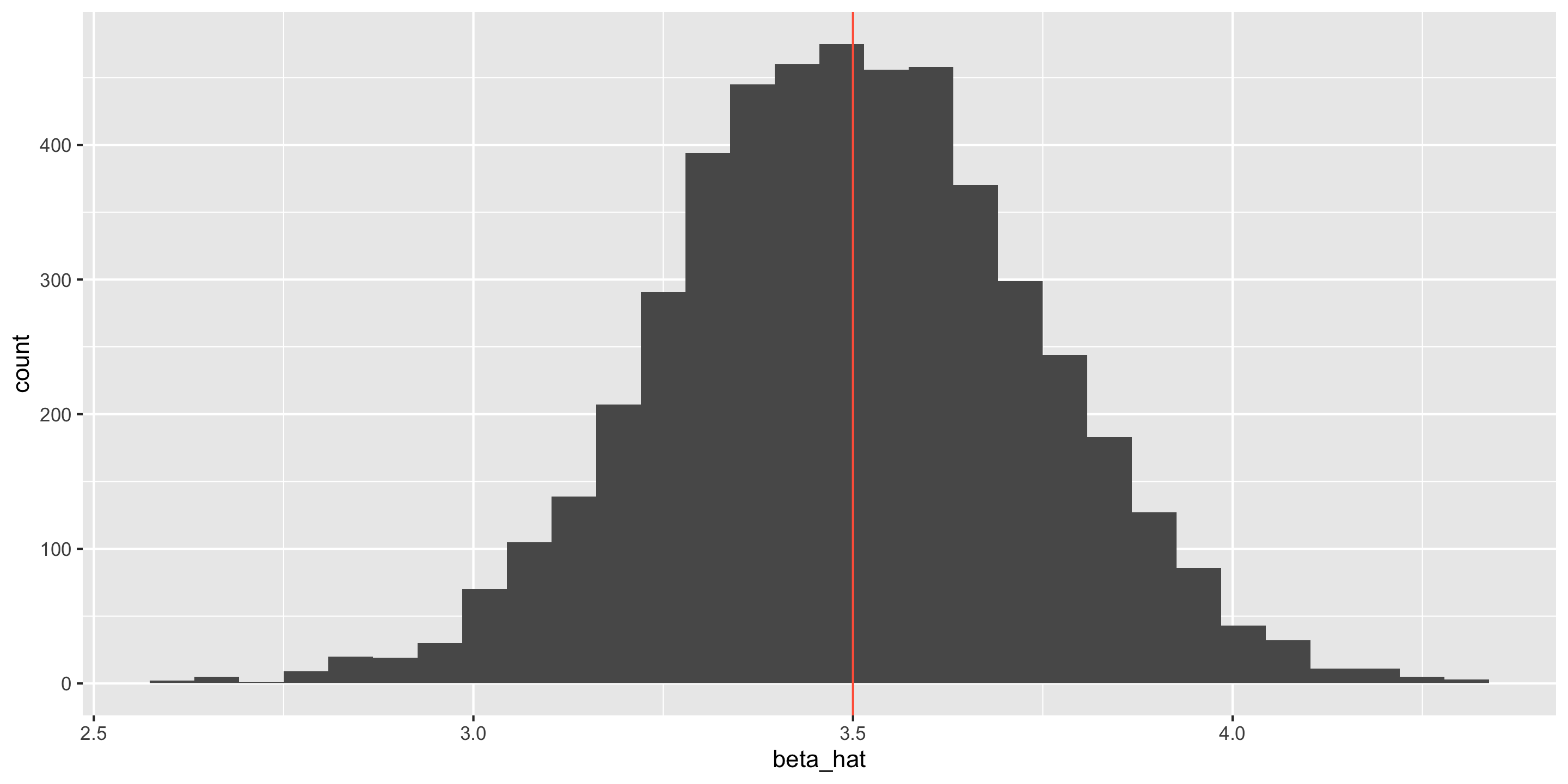
gglm::gglm()Unbiased estimation of \(\hat\beta\)
Accurate assessment of \(\mbox{SE}(\hat\beta)\)


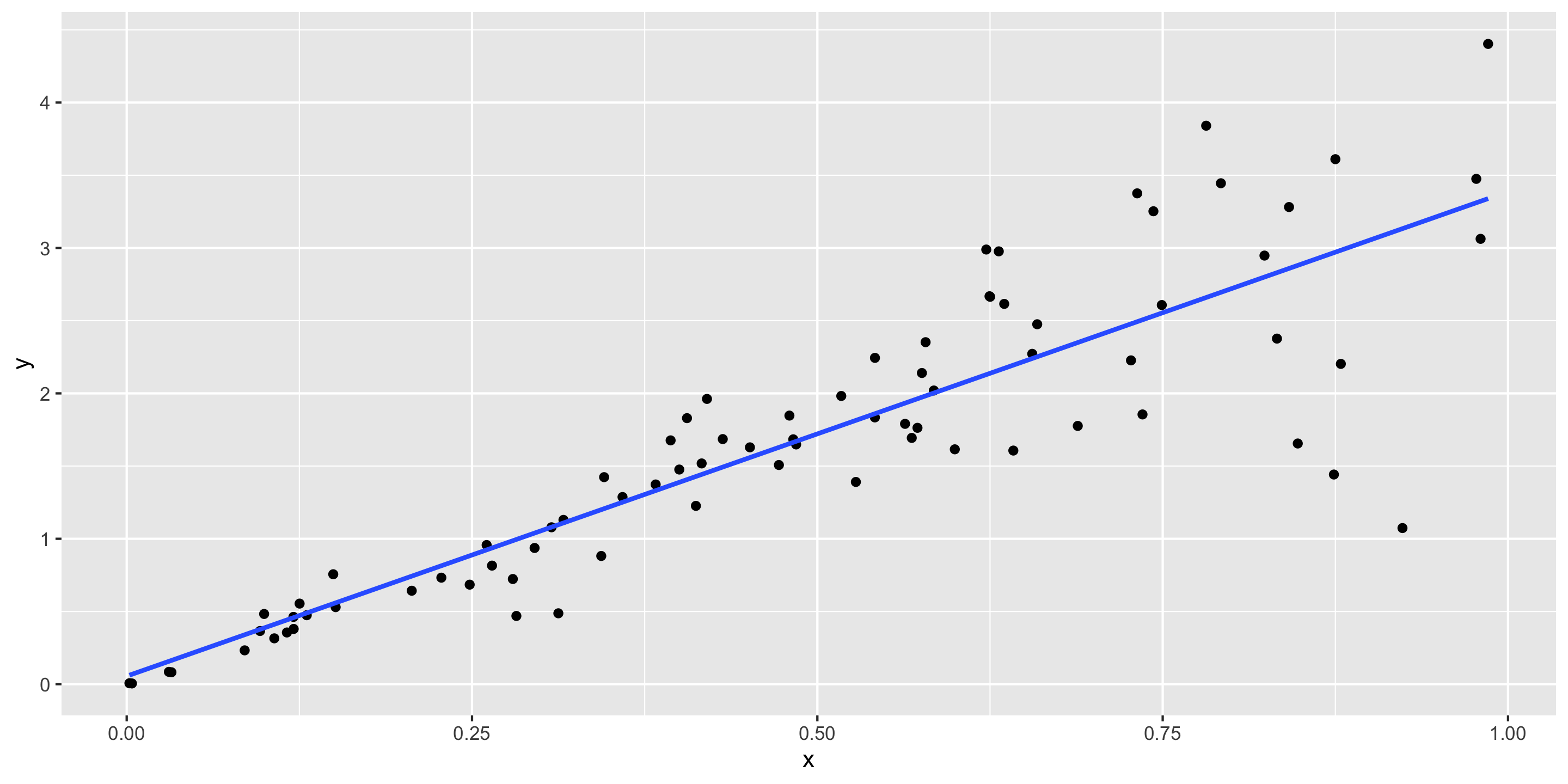
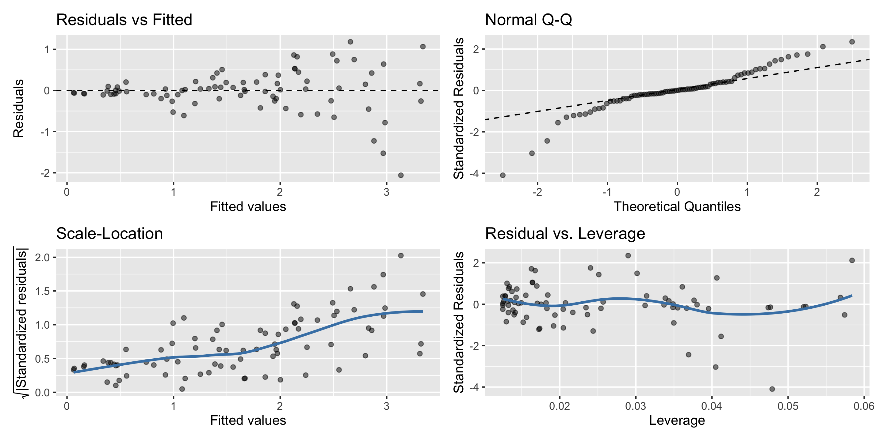
With a partner (there needs to be one computer between you), choose one of the following components of the linear model to break, then assess what goes wrong.
You can build off the code used in these slides.